 2017, Vol. 35
Institute of Oceanology, Chinese Academy of Sciences
Article Information
- LIU Yao(柳瑶), LIU Baoliang(刘宝良), LEI Jilin(雷霁霖), GUAN Changtao(关长涛), HUANG Bin(黄滨)
- Numerical simulation of the hydrodynamics within octagonal tanks in recirculating aquaculture systems
- Chinese Journal of Oceanology and Limnology, 35(4): 912-920
- http://dx.doi.org/10.1007/s00343-017-6051-3
Article History
- Received Mar. 2, 2016
- accepted in principle Apr. 5, 2016
- accepted for publication May. 10, 2016


2 Shandong Univercity, Weihai, Marine College, Weihai 264209, China
The tank is an important part of a recirculating aquaculture system (RAS) in providing the habitat for fish. It is also a part of the pre-treatment of wastewater for which the rate of removal of large particles determines the load and efficiency of wastewater treatment of the system (Timmons et al., 2002). Most studies on tanks have focused on different types (Davidson et al., 2004; Labatu et al., 2007; Prussi et al., 2014), the inlet and outlet flow structures (Vantoever, 1997; Sveier et al., 1999; Summerfelt et al., 2009; Venegas et al., 2014), and the distribution of velocity and dissolved oxygen. Several studies looked at the influences of velocity on behavior, growth, and metabolism (Leon, 1986; Rosenthal, 1987; Watten and johnson, 1990; Ross et al., 1995).
While these studies demonstrated the hydrodynamics of RAS tanks, most were concerned with the velocity distribution. There were few studies about the rates of particle removal, the existence of still-water regions with low velocity, and particle sedimentation (Davidson and Summerfelt, 2004; Couturier et al., 2009; Carvalho et al., 2013). In particular, there has been no study on particle removal and still-water regions in octagonal tanks, which are widely used in China for their rotating flows, ease of construction, and greater space utilization of the total plant compared with circle tanks. As China aquaculture produces more than 60% of the world's farmed fish (Aquaculture Research Group, Fisheries, Ministry of Agriculture, China, 2006), it is necessary to study water velocity profiles, rates of particle removal, and still-water regions. These basic aspects of the hydrodynamics in octagonal tanks supported the design and optimization of tanks that would further promote the large-scale, automation and aquacultural welfare of RASs.
To date, computational fluid dynamics (CFD) has been widely used in determining the velocity distributions in tanks (Huggins et al., 2005; Vuthaluru et al., 2009; Masaló and Oca, 2014; Venegas et al., 2014). There were a few simulation studies concerning the actual production conditions in tanks such as rates of particle removal, still-water regions, the mixing of soluble nutritive salts, and the influence of fish activity on the hydrodynamics. In particular, the turbulence model, the multi-phase model, and the diffusion model were crucial to the simulation result (Cheng and Zhu, 2005). Proper modeling reduced significantly the error between simulation and experiment. Further, the application of CFD would promote the hydrodynamics of tanks.
In this study, the k-ε realizable turbulence model and the discrete phase model (DPM) were applied to describe the velocity distribution and rate of particle removal. To our knowledge, there is no study regarding the application of DPM to the rate of removal of particles from octagonal tanks. The objectives of this study were (1) to obtain the velocity distribution and the rate of particle removal and (2) to obtain suitable models (realizable k-ε turbulence model and DPM) that describe the hydrodynamics in octagonal tanks. This study indicates the technological benefits of octagonal tanks applied in production, and moreover provides a numerical method for the design and optimization of tanks, which ultimately promotes CFD as a tool to be widely used in RAS research.
2 MATERIAL AND METHOD 2.1 Full-scale set upA RAS has been running in the commercial production of turbot and grouper at Shandong Oriental Ocean Company, Yantai, China. The system is constructed of seven main units (Fig. 1). The water from the dual-drain design tank flows through separators and the supernatant is then piped to an automatic inclined-belt filter. The water is pumped to foam fractionators, which are connected to the ozone contact chamber and on to a series of submerged biofilters which are filled with plastic media and porous biofilter media. Finally, the water is passed through UV light and a dissolved oxygen contact unit back to the tanks.

|
| Figure 1 Recirculating aquaculture system for turbot The units are: 1. twelve culture tanks; 2. separators for removing solids from bottom flow; 3. automatic inclined-belt filter for coarse solid removal; 4. foam fractionators; 5. ozone contact chamber; 6. four submerged biofilters; 7. liquid oxygen chamber. |

|
| Figure 2 Geometry of an octagonal tank rended by FLUENT software a. 1: inlet pipe; 2: particle entrapment; 3: main outlet pipe for overflow; 4: secondary outlet pipe for bottom flow; b. inlet pipe; c. waterline dual-train design. |

|
| Figure 3 Computational grid for the 34 m3 octogonal tank used in hydrodynamics simulations |
All the tanks are octagonal in shape, each with an operational volume of 34 m3. This system contains 12 6-m-diameter 'waterline-type' dual-drain culture tanks. These culture tanks are operated at a depth of 1.1 m, to yield a diameter-to-water depth ratio of 5.5:1. The total water volume of the system is 440 m3, which is cycled 12 times per day; that is, every 2 h the tank water is completely exchanged. Approximately 7% of the total flow is discharged through a drain located at the bottom center of the culture tank. The overflow is piped into the top of the outer tube and then drained off to the inner pipe. The bottom flow containing most of the total waste solids passes through a particle entrapment unit, and then drained into the separator. The velocity flow through the inlet pipe was determined by measuring the volume of water filling a bucket in a specific time; in this system, the velocity through the inlet pipe was 0.88 m/s. To ensure steady flow during the determination, the RAS had been running for 48 h prior to the measurement.
2.2 Experimental methodsThe water velocity in the tanks was measured using an acoustic Doppler profiler (Aquadopp Profiler-1 MHz, Nortek Intl., Rud, Norway). For the profiler, the 30 cm of water beneath the surface is a still-water zone and its smallest measuring interval is 50 cm. Hence the smallest depth at which velocity can be measured is 80 cm. Also, the probe submerged in the water needed at least 2 cm of water depth. The total water depth in the octagonal tank is 100 cm, hence velocities were measured at a depth of 82 cm over a plane parallel to the water surface, specifically, the cross-section at z=0.18 m. This plane was sectioned equally by six radial lines, and measurements were taken at 12 points along every line at 43-cm intervals. At each point 10 velocities readings were taken, and then averaged to give the final experimental value. Finally, the experimental data was processed using Matlab to generate a contour map of the velocities. To simplify experimental conditions and reduce the error, no fish were present during readings.
The waste solid mainly included feces and uneaten food, for which the mean density was approximately 1.19 kg/m3 (Chen et al., 1993). In this study, for particles to be moved, we chose different diameters (1, 3, 5, and 10 mm) of fish feed (Great Seven Biotech Co., Qingdao, China), of density 1.15 kg/m3. Particles with a total mass of 250 g were released from the water surface with an initial velocity of 0 cm/s at the midpoint of the side length and 0.5 m near to the wall within tanks (Fig. 1). All particles drained from the tanks are assumed to flow into the separator. A screen collector is placed in the separator to capture the particles drained from the tanks in a 10-min period. A total dry weight of 94 g of particles was recovered for every 100 g of fish feed after 12 h in the drying oven at 75℃. These collected particles were dried under the same conditions. From the known dry weight, the weight of water from the collected particles in the fish feed can then be calculated. Again, with no fish in the tank, the experimental conditions simplify in regard to the determination of the rate of particle removal. Nonetheless, swimming fish agitate solids and thereby promote particle removal.
2.3 Numerical approach 2.3.1 Governing equationsComparing standard and RNG k-ε turbulence models, the latter model is more suitable for high time-averaged strain rates that are commonly used in different types of flow simulations such as rotating uniform shear flow, free flow including jet flow and mixed flow, pipe flow, boundary-layer flow, and separated flow (Wang, 2004). The flow in octagonal tanks includes a rotating flow and sedimentation, therefore the RNG k-ε turbulence model was applied. The governing equations are:
Continuity equation:
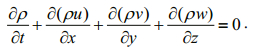 (1)
(1)Momentum equations:
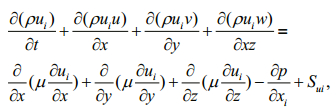 (2)
(2)where ρ and μ are the density and viscosity of the fluid; t is the elapsed time; u, v, w are the velocity components along the x, y, z axes; p is the pressure; i=1, 2, 3, ui=u1, u2, u3=u, v, w, xi=x1, x2, x3=x, y, z; Sui is the source term for the momentum equation, Sui=Fxi+Sxi, Sxi=0 for incompressible fluid; Fxi is the force of gravity, and hence Su=Fx=0, Sy=Fy=0, Sw=Fz= -ρg.
Realizable k-ε model:
k equation:
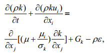 (3)
(3)ε equation:
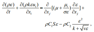 (4)
(4)where Gk is the turbulent kinetic energy generated by the average velocity gradient; C1=max[0.43, η/(η+5)], η=Sk/ε, σk=1.0, σε=1.2, C1=1.44, C2=1.9.
2.3.2 Discrete Phase ModelThe DPM is more suitable for studying particle grading and separation. The interaction of particles and the influence of particles on the continuous phase are ignored if the volume fraction of solids is less than 12% (Yu, 2008). In our study, the coupling between phases is ignored if the volume fraction is less than 1%. The trajectory of a particle is traced in the Lagrangian formulation using the integral of the differential equation of motion for a particle under applied forces. The balance equation for the particle under the given forces is
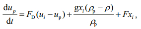 (5)
(5)where FD(ui-up) is the drag acting on a particle per unit of weight, FD=(18μ/ρpdp2)(CDRe/24); u the velocity of the fluid; up the velocity of the particle; μ the viscosity of the fluid; ρ the density of fluid; ρp the density of the particle; Fxi other forces; dp the diameter of the particle; Re Reynolds Number, Re=(ρdpIup-uI/μ).
2.3.3 Mesh grids, boundary conditions, and numerical algorithm methodThe quality of the mesh is a critical aspect of a simulation. A series of tests were run to find the most appropriate. Finally, a tetrahedral mesh for the octagonal tank was adopted, and the parts of complex structure were locally densified. The total number of cells was 0.9 million. The minimum volume was 10-9 m3 and the maximum aspect ratio was 50. The minimum orthogonal quality was 0.1.
The boundary condition at the water inlet sets the inlet velocity at 0.88 m/s. There are two outlet pipes for which the outlet velocity is set from boundary conditions. No-slip wall boundary conditions are set for the rest of the tank. The turbulence intensity (I) and the hydraulic diameter (DH) of the inflow are set as I=0.16 Re-0.125 and DH=Dinlet, respectively. The interaction of the phases is ignored in the DPM; the particles were released from the water surface with an initial velocity of 0 cm/s at the midpoint of the side length and 0.5 m near to the wall within tanks (Fig. 1).
The three-dimensional numerical model was subdivided and the governing equations discretized using the finite volume method in FLUENT 6.3. The governing equations were solved with the pressurebased solver in a first-order, implicit, steady formulation. The pressure-velocity coupling was calculated using the SIMPLEC algorithm. The discretization scheme uses the first-order upwind scheme. Convergence of the simulation was deemed achieved when the residuals for all variables were less than 0.000 1.
3 RESULT AND DISCUSSION 3.1 Velocity distribution within the octagonal tank 3.1.1 Contour of velocityThe velocity distribution at the z=0.18 m crosssection of octagonal tanks is shown in Fig. 4. Comparing simulation values with experiment values, we conclude that the trend in the distributions is similar; specifically, velocities are lower when closer to the center and have a minimum around the center of the drain. Nevertheless, there are several obvious differences. First, the velocity is more uniform in the simulation. This may be because the simulation evolves in an ideal state, whereas in the actual experiment there is a greater variation in the external disturbances, giving rise to experiment errors and flow instability. The velocity distribution from the simulation has the following pattern: L≤1.5 m, v≤15 cm/s; 1.5 m≤L≤2.2 m, 15 cm/s≤v≤20 cm/s; 2.2 m≤L≤3.0 m, 20 cm/s≤v≤25 cm/s. There is a small oval area near the walls where the range of velocities is 25 cm/s≤v≤35 cm/s. The mass-weight average velocity is 16.1 cm/s for all tanks in the simulation. Second, the velocity along the direction of inflow is quite high, reaching up to 80 cm/s, which possibly results in high energy losses causing wall abrasion. This should improve with the optimization of angle, number, and direction of the inlet pipe. These do not show up in experimental data because of device limitations on measurements. Third, the velocity at the tank center in the experiment is higher than that in simulations. This may be because there is a vortex at the center of the tank, which affects instrument readings. Finally, the corner velocity (average ≥15 cm/s) is lower in areas along the walls, but still higher than the velocity at the center. Hence the mixing of water in the corners is not as bad as for rectangular tanks, possibly because the obtuse corners of an octagon appear smoother like a circle compared with a square corner. Thus, in general, the velocity distributions are similar for both simulation and experiment. The results of both are consistent as can be assessed intuitively from the contour maps of velocity. Additionally, the results from simulations provide a more comprehensive view of the hydrodynamics, which are consistent with that encountered in the study by Wei (2013) for circular tanks.

|
| Figure 4 Contour maps of the magnitude of velocity for a 34 m3 octagonal tank obtained from experimental data and simulation at cross section z=0.18 m with water inlet velocity of 0.88 m/s |
The velocity distribution along one of the six radial lines in z=0.18 m cross-section (Fig. 5) shows that, for both experiment and simulation, the velocity is lower closer to the center of tank. Additionally, the central velocity in the experiment is higher than in the simulation. In particular, the difference in velocity is larger if the velocity is less than 15 cm/s, possibly because the accuracy of the simulation is insufficient. Generally, the discrepancy is larger if the simulation is run with lower initial velocities (Liu et al, 2014). Moreover, we see that the velocity decreases significantly within 10 cm of a wall because shearing forces exists between the viscous fluid and the wall in simulations. This is consistent with the rotational velocity distribution of the circular tank at different cross sections reported by Yu et al. (2012). The accuracy of the simulation is validated by the experiment. Generally, if the mean relatively error is less than 30%, then the simulation is considered consistent with the experiment; here the relative error is given by |simulation-experiment|/ experiment×100%. The average mean relative error (MRE) is the average of all relative errors. Between experiment and simulation, the MRE for velocity is 18% over the z=0.18 m cross-section which is less than 30%. Hence, we conclude that there is a broad consistency between experiment and the threedimensional steady-state simulation employing the tetrahedral mesh and the realizable k-ε model.

|
| Figure 5 Velocity distribution along one of the six radial lines at cross section z=0.18 m |
These parameters and models can be used in describing the self-cleaning capability and optimization of octagonal tanks. Almansa et al. (2012) indicated that 22-cm turbots distributed homogenously with normalized episode velocities of 0.33-0.46 BL/s (0.073-0.10 m/s), avoided swimming at 0.58 BL/s (0.13 m/s), and were unable to maintain their positions at a velocity of 0.98 BL/s (0.22 m/s). In this study, the water velocity was lower than 20 cm/s with a radius of 2.2 m of the tank center, conditions for which are good for tank self-cleaning and fish health.
3.2 Self-cleaning of octagonal tanks 3.2.1 Validation of self-cleaningFrom the trajectories of particles of different sizes (Fig. 6), we conclude that smaller particles follow the streamlines of water more closely and hence their hydrodynamic retention time is longer. Particles of diameter 1, 3, and 5 mm were drained from the tank after an elapsed time of 451 s (7.5 min), 171 s (2.9 min), and 114 s (1.9 min), respectively. The longer the particles are retained in the tank, the worse the water quality is, and the more harm they do to fish gills. For a circular tank, Wei (2013) reported much shorter residence times of 275 s (4.6 min) and 58 s (1 min) for 1-mm and 3-mm particles, respectively, with a 0.8-m/s water inlet velocity. This is possibly because of the tank geometry and a dual-directional inflow. Comparing the results from simulation and experiment regarding the rate of removal for the different-sized particles, i.e., 1, 3, and 5 mm, we conclude that the rate of removal of the different sized particles correlates 100% with those in the simulation. However, the rate of removal of particles is calculated by {[Mdry weight+Mdry weight/(94×100-94)]/250}×100% in experiment, which is separately 89%, 91%, 92.5% for the 1-, 3-, 5-mm diameter particles, respectively. There are several reasons why values are smaller for experiment than for simulations. First, in the experiment, residual particles remain in the tank following collection. Smaller particles are better entrained with the streamlines of water, and hence more particles remain in the tank. Second, there are fewer particles escaping from the filter screen. Third, the stability of fish feed in water is not ideal in that small parts leach into the tank water. For the rate of removal for the three sizes of particles, the error ranges between 8% and 11% for simulation and experiment. The conclusion is that, regarding selfcleaning tanks, the DPM simulation produces results consistent with those from experiment data. Moreover, the DPM is useful in optimizing tank operations.

|
| Figure 6 Trajectory and residence times of different-sized particles: a) 1 mm, b) 3 mm, c) 5 mm, in an octagonal tank with initial inflow velocity of 0.88 m/s |
The trajectories of three different-size particles released from inlet pipe in the third corner are shown in Fig. 7. Particle sedimentation in the corners is a controversial point in octagonal tanks. These trajectories were simulated using the realizable k-ε turbulence model and the DPM with releases from all corners of the tank. The conclusion is that the trajectories are similar for each corner apart from the different initial positions. Hence only the trajectories of particles from the third corner are shown. We see that particles of diameter 3, 5, 10 mm flow along the wall. The 10 mm-diameter particle is drained from the tank after 154 s (2.6 min) (Fig. 7c). However, the 3 mm and 5-mm-diameter particles remain in the tank after 540 s (9 min) (Fig. 7a) and 750 s (12.5 min) (Fig. 7b), respectively. The sediment location is a small area between the inlet pipe and the tank wall where the small particles are re-suspended and cannot be drained away (Fig. 7a and b), possibly because accelerations are strong that result in a vortex with negative pressure. This can be adjusted by altering the angle and position of the inlet pipe. Thus, with a 0.88-m/s inflow in a 34-m3 octagonal tank, particles smaller than 5-mm in diameter tend to gather at the area between the inlet pipe and the tank wall. There is no sediment in other corners. Tvinnereim (1994) reported that square tanks having a total side length of a with cut corners of size a/5 could avoid still-water zones, whose ratio of diameter to height was 2:1. However, square, rectangular, and raceway tanks avoid such zones in different ways (Lekang, 2013). As this study was done with no fish present, it is possible that these zones can be avoided through the activities of fish because the resulting agitation is important in particle removal (Timmons et al., 2002).

|
| Figure 7 The pathline and residence time of different particles released from the third corner from inlet pipe a: 3 mm, b: 5 mm, c:10 mm. |
The velocity distribution and self-cleaning of a full-scale octagonal tank was studied by combining simulations with experiments. We obtain the following conclusions.
Using the realizable k-ε model for turbulence modeling, we found that the three-dimensional steady simulation outputs are consistent with experiment data. The mean relative error for the velocity in the z=0.18 m cross-section is 18%.
Using the DPM to simulate trajectories of particles in the tank, the error between simulation and experiment for the rate of particle removal is between 8% and 11%. Moreover, small particles of less than 5 mm in diameter tend to gather in an area between the inlet pipe and the tank wall under a 0.88-m/s inflow. There was no sedimentation in other corners.
Comparing the contour map of velocities from simulation results with those of experimental data, we found the simulation output to be consistent with experimental results. Additionally, the results are more comprehensive in simulations in terms of velocity uniformity over the entire tank, the high water velocity along the direction of inflow, the minimum velocity in the center of the tank, and the high corner velocity and strong mixing.
The CFD results are significant for revealing the hydrodynamics within a RAS and the optimization of its parameters. However, the accuracy of the simulation needs to be improved to reflect actual production conditions, which continues to be a prominent theme in RAS research.
| Almansa C, Reig L, Oca J, 2012. Use of laser scanning to evaluate turbot (Scophthalmus maximus) distribution in raceways with different water velocities. Aquacultural Engineering, 51: 7–14. Doi: 10.1016/j.aquaeng.2012.04.002 |
| Carvalho R A P L F, Lemos D E L, Tacon A G J, 2013. Performance of single-drain and dual-drain tanks in terms of water velocity profile and solids flushing for in vivo digestibility studies in juvenile shrimp. Aquacultural Engineering, 57: 9–17. Doi: 10.1016/j.aquaeng.2013.05.004 |
| Chen S L, Timmons M B, Aneshansley D J, Bisogni Jr J J, 1993. Suspended solids characteristics from recirculating aquacultural systems and design implications. Aquaculture, 112(2-3): 143–155. Doi: 10.1016/0044-8486(93)90440-A |
| Cheng Y, Zhu J X, 2005. CFD modelling and simulation of hydrodynamics in liquid-solid circulating fluidized beds. The Canadian Journal of Chemical Engineering, 83(2): 177–185. |
| Couturier M, Trofimencoff T, Buil J U, Conroy J, 2009. Solids removal at a recirculating salmon-smolt farm. Aquacultural Engineering, 41(2): 71–77. Doi: 10.1016/j.aquaeng.2009.05.001 |
| Davidson J, Summerfelt S, 2004. Solids flushing, mixing, and water velocity profiles within large (10 and 150 m3) circular 'Cornell-type' dual-drain tanks. Aquacultural Engineering, 32(1): 245–271. Doi: 10.1016/j.aquaeng.2004.03.009 |
| Huggins D L, Piedrahita R H, Rumsey T, 2005. Use of computational fluid dynamics (CFD) for aquaculture raceway design to increase settling effectiveness. Aquacultural Engineering, 33(3): 167–180. Doi: 10.1016/j.aquaeng.2005.01.008 |
| Labatu R A, Ebeling J M, Bhaskaran R, Timmons M B, 2007. Hydrodynamics of a large-scale mixed-cell raceway(MCR):experimental studies. Aquacultural Engineering, 37(2): 132–143. Doi: 10.1016/j.aquaeng.2007.04.001 |
| Lekang O I, 2013. Aquaculture Engineering. WileyBlackwell Publishing, Oxford, UK228p. |
| Leon K A, 1986. Effect of exercise on feed consumption, growth, food conversion, and stamina of brook trout. The Progressive Fish-Culturist, 48(1): 43–46. Doi: 10.1577/1548-8640(1986)48<43:EOEOFC>2.0.CO;2 |
| Liu Y, Song X F, Liang Z L, Peng L, 2014. Application of CFD modeling to hydrodynamics of CycloBio fluidized sand bed in recirculating aquaculture systems. Journal of Ocean University of China, 13(1): 115–124. Doi: 10.1007/s11802-014-2029-3 |
| Masaló I, Oca J, 2014. Hydrodynamics in a multivortex aquaculture tank:effect of baffles and water inlet characteristics. Aquacultural Engineering, 58: 69–76. Doi: 10.1016/j.aquaeng.2013.11.001 |
| Prussi M, Buffi M, Casini D, Chiaramonti D, Martelli F, Carnevale M, Tredici M R, Rodolfi L, 2014. Experimental and numerical investigations of mixing in raceway ponds for algae cultivation. Biomass and Bioenergy, 67: 390–400. Doi: 10.1016/j.biombioe.2014.05.024 |
| Ross R M, Watten B J, Krise W F, DiLauro M N, Soderberg R W, 1995. Influence of tank design and hydraulic loading on the behavior, growth, and metabolism of rainbow trout(Oncorhynchus mykiss). Aquacultural Engineering, 14(1): 29–47. Doi: 10.1016/0144-8609(94)P4425-B |
| Summerfelt S T, Sharrer M, Gearheart M, Gillette K, Vinc B J, 2009. Evaluation of partial water reuse systems used for Atlantic salmon smolt production at the White River National Fish Hatchery. Aquacultural Engineering, 41(2): 78–84. Doi: 10.1016/j.aquaeng.2009.06.003 |
| Sveier H, Wathne E, Lied E, 1999. Growth, feed and nutrient utilisation and gastrointestinal evacuation time in Atlantic salmon (Salmo salar L.):the effect of dietary fish meal particle size and protein concentration. Aquaculture, 180(3-4): 265–282. Doi: 10.1016/S0044-8486(99)00196-9 |
| Timmons M B, Ebeling J M, Wheaton F W, Summerfelt S T, Vinci B J. 2002. Recirculating Aquaculture Systems. 2nd edn. NRAC Publication No. 01-002, Northeastern Regional Aquaculture Center, Cayuga Aqua Ventures, Ithaca, NY. p. 130-185. |
| Timmons M B, Summerfelt S T, Vinci B J, 1998. Review of circular tank technology and management. Aquacultural Engineering, 18(1): 51–69. Doi: 10.1016/S0144-8609(98)00023-5 |
| Tvinnereim K. 1994. Hydraulisk utforming av oppdrettskar. Brukerpport. SINTEF Report STF60A94046. (in Norwegian). |
| Vantoever W J. 1997. Water treatment system particularly for use in aquaculture: US, US Patent No. 5593574. 1997-01-04. |
| Venegas P A, Narváez A L, Arriagada A E, Llancaleo K A, 2014. Hydrodynamic effects of use of eductors (JetMixing Eductor) for water inlet on circular tank fish culture. Aquacultural Engineering, 59: 13–22. Doi: 10.1016/j.aquaeng.2013.12.001 |
| Vuthaluru R, Tade M, Vuthaluru H, Tsvetnenko Y, Evans L, Milne J, 2009. Application of CFD modelling to investigate fluidized limestone reactors for the remediation of acidic drainage waters. Chemical Engineering Journal, 149(1-3): 162–172. Doi: 10.1016/j.cej.2008.10.014 |
| Wang F J, 2004. Analysis Computational Fluid Dynamics-Principle and Application of CFD Software. Tsinghua University Press, Beijing, Chinap.124-125. |
| Watten B J, Johnson R P, 1990. Comparative hydraulics and rearing trial performance of a production scale crossflow rearing unit. Aquacultural Engineering, 9(4): 245–266. Doi: 10.1016/0144-8609(90)90019-V |
| Wei W, 2013. Numerical Simulation and Structure Optimization of Circular Culture Tank for Recirculating Aquaculture Systems. Guangdong Ocean University, Zhanjiang. |
| Yu G Y, Wei W, Wang X Z, He Z, Yan F L, 2012. Numerical simulation and verification on flow-field distribution in 'Cornell-type' dual-drain culture tank. Fishery Modernization, 39(6): 10–14. |
| Yu Y, 2008. FLUENT Introductory and Advanced Tutorial. Beijing Institute of Technology Press, Beijing, Chinap.45-153. |