 2017, Vol. 35
Institute of Oceanology, Chinese Academy of Sciences
Article Information
- LIANG Jianjun(梁建军), DU Tao(杜涛), HUANG Weigen(黄韦艮), HE Mingxia(贺明霞)
- Numerical investigation of wake-collapse internal waves generated by a submerged moving body
- Chinese Journal of Oceanology and Limnology, 35(4): 967-977
- http://dx.doi.org/10.1007/s00343-017-6041-5
Article History
- Received Feb. 5, 2016
- accepted in principle Apr. 26, 2016
- accepted for publication Jun. 16, 2016


2 College of Oceanic and Atmospheric Sciences, Ocean University of China, Qingdao 266003, China;
3 Second Institute of Oceanography, State Oceanic Administration, Hangzhou 310012, China
Internal waves generated by a submerged moving body in a stratified fluid represent one of the significant branches of stratified flow dynamics, and are closely related to military applications. In general, the waves can be classified into three types. The first is generated by a combined volume flux effect contributed by a body and its attached flow structure, referred to as a lee wave. The second is generated by gravitational collapse of a mixed region in the body wake, referred to as a wake-collapse internal wave. The third is generated by the collapse of large-scale turbulent structures in the body wake, referred to as a wake random internal wave (Wei et al., 2009). A literature survey shows that the first and third types have received considerable attention but reports about the second type remain scarce (Gilreath and Brandt, 1985; Bonneton et al., 1993; Wei et al., 2009; Brandt and Rottier, 2015). Summarizing the available research results shows that laboratory studies only confirm the generation of the second type of internal waves, without detailed analysis of their properties (Schooley and Stewart, 1963; Gilreath and Brandt, 1985). Even numerical studies do not directly consider the essential effects of both body geometry and propeller forcing (Chernykh et al., 2004). Thus, it is still unclear whether wake-collapse internal waves can be generated by a propeller-driven body in oceanic stratified conditions, and what the wave properties are if they are generated. To answer these two questions, the present study simulates turbulent wakes generated by a propeller-driven body in a linearly stratified ocean, and explores the generation and properties of wake-collapse internal waves.
The paper is organized as follows. A newly developed numerical model and corresponding solution method are given in Section 2. Model initialization is described in Section 3. Section 4 contains numerical results with different body speeds and stratification magnitudes. Conclusions are given in Section 5.
2 NUMERICAL MODEL AND NUMERICAL SOLUTION METHOD 2.1 Numerical modelThe newly developed numerical model consists of Reynolds-averaged Navier-Stokes equations, a propeller body-force model, and turbulence closure model.
2.1.1 Reynolds-averaged Navier-Stokes equationsThe Reynolds-averaged Navier-Stokes equations are used to describe the situation in which a propellerdriven body moves with constant speed in an initially quiescent medium. A similar situation, in which a thin vertical barrier moves uniformly in such a medium, has been studied by Houcine et al. (2012). From their numerical results, they identified transient internal waves and stationary lee waves. In the present study, the body was geometrically similar to the classic Suboff model constructed by the Defense Advanced Research Projects Agency in the USA. The Suboff model is composed of an axisymmetric hull, a sail, and four stern appendages. To mimic a realistic submerged body, the size of the model is enlarged 25 times, to have an overall length of 108.9 m and maximum diameter of 12.7 m. In practice, propellerinduced flow is three-dimensional, highly unsteady and turbulent, so a very small time step and spatial resolution are required to capture the detailed flow field around a propeller. This results in a very high computational cost (Phillips et al., 2009). Such treatment is necessary when propeller performance and efficiency are the only interest. However, when the turbulent wake of a propeller-driven body is the interest, the propeller effect is normally represented by a body-force model (Schetz and Favin, 1979; Stern et al., 1988; Paterson et al., 2003; Alin et al., 2010). The common method of implementing a body-force model is directly adding source terms that represent the propeller forcing in the momentum equation. The relevant body-force model used herein is discussed in Section 2.1.2.
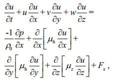
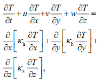
The momentum equation uses the Boussinesq approximation; that is, the effect of density variation is only considered in the gravity term. Further, the density of seawater is assumed to be a function of temperature only, and the Coriolis force is neglected. Then, the equations of conservation of momentum, conservation of mass, temperature transport (Afanasyev and Peltier, 2001; Vlasenko et al., 2005), and state (Millero and Poisson, 1981) are
 (1.1)
(1.1)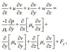 (1.2)
(1.2)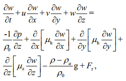 (1.3)
(1.3)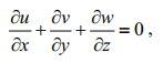 (2)
(2) (3)
(3)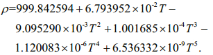 (4)
(4)Here, u, v, and w are the velocity components corresponding to x, y, and z coordinates; t is time; T is temperature; ρ is density; ρa is the initial stable density profile; ρ0 is the reference density; g is gravitational acceleration; Fx, Fy, and Fz are the components of force generated by a propeller; μh and μz are horizontal and vertical eddy viscosity coefficients for momentum; and Кh and Кz are the horizontal and vertical eddy diffusivity coefficients for temperature.
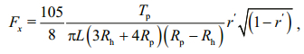
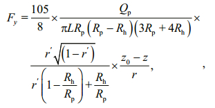
2.1.2 Propeller body-force modelIn the model, the effect of the propeller is represented by forces Fx, Fy, and Fz. According to the equation proposed by Paterson et al. (2003), these forces in Eqs.1.1-1.3 can be alternatively expressed as
 (5)
(5) (6)
(6)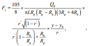 (7)
(7)where Tp represents the propeller's total thrust; Qp represents its total torque; Rh is the hub radius; Rp is the propeller radius; L is the chord length at 0.7Rp; and 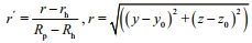
The determination of Tp and Qp in Eqs.5-7 is as follows. It is known that Tp is equivalent to the total drag F that a body experiences when moving at constant velocity without the propulsion of a propeller. Therefore, Tp can be indirectly obtained by calculation of F, which is calculated by
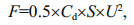 (8)
(8)where Cd is the total drag coefficient; U is the body speed; and S is the total surface area. The determination of Cd is via steady-state numerical simulation without considering propeller forcing in a homogenous fluid. Thus, substituting Cd into Eq.8 makes F known and thereby obtains Tp. After Tp is available, Qp is obtained via the following relationship (Yang et al., 2013).
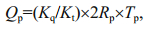 (9)
(9)where Kt is the thrust coefficient and Kq the torque coefficient.
2.1.3 Turbulence closure modelThe effects of eddy viscosity and diffusivity are included in the newly developed model. A constant coefficient turbulence model (Legg and Adcroft, 2003; Fringer et al., 2006; Chen et al., 2014) has been used in many numerical simulations of oceanic internal waves and is also used here because of its simplicity and efficiency. The characteristic horizontal eddy viscosity coefficient μh was 10-1 m2/s in the light of numerical experiments in a homogeneous fluid with the same grid. Because the horizontal eddy viscosity and diffusivity coefficients mainly depend on grid resolution (Vlasenko and Hutter, 2002), we set them to μh=Кh=10-1 m2/s. In addition, invoked by the turbulence model used by Vlasenko and Stashchuk (2007), we took the vertical eddy viscosity and diffusivity coefficients as μz=Кz=1.5×10⁻² m2/s.
2.1.4 Boundary conditionsTo ensure that the generated internal waves could not reach the boundaries in the period of interest, the computational domain of the model was dimensioned as x∈(-200, 800) m, y∈(-150, 150) m, and z∈(-300, 0) m. The center of the submerged body was located at (100.2, 0, -100) m and its front and tail were at x=45.7 m and x=154.6 m, respectively (Fig. 1). To keep the propeller-driven body fixed in the computational domain, a moving coordinate system was adopted (Guan et al., 2012; Rojanaratanangkule et al., 2012).

|
| Figure 1 Schematic diagram of computational domain |
In the experiments, no normal flux conditions were applied to the boundaries, except the one on the left. Inflow and outflow boundary conditions were specified at the left and right boundaries, respectively. Free slip boundary conditions were applied to the top and bottom boundaries, and no-slip boundary conditions at the body surface. At the side boundaries, normal velocity gradients were taken as zero. Numerical boundary conditions were applied to pressure at each boundary.
2.2 Numerical solutionThe aforementioned numerical model was solved using the open-source computational fluid software OpenFOAM. This software uses the finite-volume method and has been widely accepted by investigators for studying complex problems (Lin and Song, 2012; Flore et al., 2013; Stringer et al., 2014). In our study, discretization of the computational domain was accomplished by the SnappyHexMesh utility within the software, and the CheckMesh utility was used to guarantee that the generated grid was adequate for accurate computation. For the discretization of equations, the temporal term was discretized by the first-order implicit Euler scheme. The advection terms were discretized by a second-order upwind differencing scheme and the diffusion terms by a second-order central differencing scheme. The discretized pressure and velocity were coupled with the pressure implicit with splitting of operators algorithm. To ensure the dominance of physical dispersion over numerical dispersion and fine spatial resolution to capture key processes, a uniform step of 5 m was used for the background mesh. Then, the body surface, propeller and wake regions were refined by factors of five, six and two, respectively. To make the computation satisfy the Courant-Friedrichs-Lewy stability condition, an adaptive time-stepping technique was used to maintain the maximum Courant number at no larger than 0.5 during the entire numerical calculation.
3 MODEL INITIALIZATIONA detailed description of the parameter setup and initialization of the temperature profile in the newly developed model are given in this section.
3.1 Parameters in propeller body-force modelTo fit the enlarged body model, a new, improved propeller model was constructed based on standard seven-blade marine propeller INSEAN E1619 (Chase and Carrica, 2013), for which the primary parameters were Rp=3.275 m, Rh=0.68 m, and L=0.092 m. The location of the propeller center was (152.3, 0, -100) m, according to that prescribed in the Suboff model. We took Kt=0.2 and Kq=0.04 per the INSEAN E1619 open-water performance curve (Chase and Carrica, 2013), thereby relating Tp and Qp by
 (10)
(10)where Tp depends on U. In general, the speeds of a submerged moving body range from 1.5 to 9 m/s. Thus, we set U to 1.5, 4.5, and 7.5 m/s, which represent low-speed, middle-speed and high-speed situations, respectively. Corresponding to each speed, the Tp and Qp were obtained by steady-state numerical experiments without the propulsion of a propeller. Here, when U=1.5 m/s, Tp=15.08 m4/s2 and Qp=19.76 m5/s2; when U=4.5 m/s, Tp=119.94 m4/s2 and Qp=157.12 m5/s2; when U=7.5 m/s, Tp =319.46 m4/s2 and Qp=418.50 m5/s2.
3.2 Initial temperature profileThe model temperature profile was given by
 (11)
(11)where H=300 m is total water depth; T1 is temperature at the sea surface; and T2 is temperature at the set bed. Considering that the order of oceanic buoyancy frequency is 10-3/s to 10-2/s, we designed three temperature profiles, which represent weakly, moderately and strongly stratified oceans, respectively. Buoyancy frequencies of the three cases at the location of the body z=-100 m were 3.27×10⁻³/s, 8.66×10⁻³/s and 1.38×10⁻²/s, respectively.
4 MODEL RESULTThe input parameters of the designed numerical experiments are listed in Table 1, including the body speed, stratification magnitude, and moving depth. We use Case1 to expound the generation process and basic properties of wake-collapse internal waves, and compare Case1, Case2 and Case3 to address the effect of body speed on the wave generation and properties. We compare Case1, Case4 and Case5 to analyze the effect of stratification on the wave generation and properties.
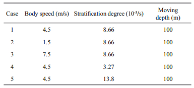
Figure 2 shows distributions of horizontal velocity profiles overlaid by isopycnal surfaces at t=5, 11, 12, and 15 s in the Case1 experiment, respectively. It is seen from Fig. 2a that the turbulent wake expands uniformly in the vertical from the initial time to t=5 s, with a boundary shape of symmetric wedge type. Meanwhile, density within the wake is strongly mixing. Afterward, the wake continues expanding because the turbulent diffusive force is still stronger than the buoyancy force, and expands to its maximum extent at t=11 s (Fig. 2b). At t=12 s, wake collapse occurs and leads to the initial generation of internal waves under the inhibiting effect of buoyancy force (Fig. 2c). At t=15 s, the internal wave has escaped from the wake and begins to propagate downstream (Fig. 2d).

|
| Figure 2 Horizontal velocity profiles overlaid by isopycnal surfaces in turbulent wakes at t=5 s (a), t=11 s (b), t=12 s (c), and t=15 s (d) in Case1 |
Figure 2 clearly illustrates the entire generation process of wake-collapse internal waves; that is, wake development, collapse and generation. The generation process basically agrees with the laboratory findings of Schooley and Stewart (1963).
4.2 Basic propertiesFigure 3a-b depicts contours of density at t=20 s and 50 s in the Case1 experiment. This shows that the entire wave disturbance is almost entirely within the section between z=-110 m and z=-85 m. Zoomed views (Fig. 3c-d) of this section at t=20 s and 50 s show that the waveform in that period was essentially maintained. Moreover, displacement of isopycnal surfaces was bounded by z=-100 m, above which those surfaces were displaced upward and below which they were displaced downward. This structure indicates that the internal wave is of second-mode character (Kao and Pao, 1980; Yang et al., 2010).

|
| Figure 3 Contour plots of density across entire depth at t=20 s (a) and t=50 s (b) zoomed views of density plots from -110-m to -85-m depths at t=20 s (c) and t=50 s (d) in Case1 |
To ensure that the generated internal waves are of second-mode character, consider the current field at t=50 s (Fig. 4a). The section of Fig. 4a between 375 and 390 m clearly shows symmetrical circulating cells, which coincide well with observed current (Fig. 4b) and analytical current (Fig. 4c) characteristics of a second-mode internal waves. However, given that the crucial property of internal waves is phase speed, we determined that speed numerically according to locations labeled by black dashed lines in Fig. 3, which show the wave center for comparison with the theoretical one. The theoretical phase speed was calculated via the three-layer formula of Yang et al. (2010) because the numerical result showed that the generated internal wave resembled an interfacial one in a three-layer system; the theoretical result was 0.15 m/s. The numerical phase speed was 0.17 m/s. This agreement between the theoretical and numerical phase speeds confirms that the internal wave is indeed a second-mode internal wave.

|
| Figure 4 Current field at t=50 s in Case1 (a) current field observed in the laboratory (b) and theoretical streamlines (c) of a second-mode internal wave (Kao and Pao, 1980) |
A comparison among numerical results of Case1, Case2 and Case3 shows that the body speed has a strong effect on the generation of wake-collapse internal waves. In Case2, the model result did not show discernible such waves (Fig. 5). The reason, according to the laboratory results of Lin and Pao (1979), is that the buoyancy force strongly inhibits turbulent motion because of a reduction of propeller forcing in the initial stage, so that mixing in the wake is greatly reduced and there was no apparent wake collapse in the model results. Therefore, the wakecollapse internal wave was so weak that it could not be observed. This leads to the conclusion that evident wake-collapse internal waves are generated only when the speed is greater than some critical value. In Case3, the model result clearly shows that generation strength increased relative to that of Case1 and that generation time was at t=8 s (Fig. 6), 4 s earlier than in the latter case. This earlier generation is attributed to the greater speed of the moving body. Because of this faster body motion, the body is able to create more vigorous turbulent motions. Therefore, there is an earlier large-scale isopycnal overturning event near the wake boundaries, which produces an earlier wake collapse under the influence of buoyancy force.

|
| Figure 5 Distribution of horizontal velocity, overlaid by isopycnal surfaces at t=60 s in Case2 |

|
| Figure 6 Distribution of horizontal velocity, overlaid with isopycnal surfaces at t=8 s in Case3 |
Because there was no perceptible wake-collapse internal wave in the Case2 experiment, the results from Case1 and Case3 were compared. This comparison demonstrated two notable effects of body speed on the wave properties. The first was that as body speed increased, stronger turbulent mixing caused the generation of a second-mode internal wave of larger amplitude. The wave amplitude, defined as the maximum isopycnal displacement relative to its equilibrium level, was ~1.0 m in Case1, in which the body speed was 4.5 m/s (Fig. 3b), while the wave amplitude was 1.4 m in Case3, in which the body speed was 7.5 m/s (Fig. 7b). The second effect was that the difference of body speed produced a different waveform evolution. Figure 3 shows that the waveform had almost no change from t=20 s to t=50 s in Case1, whereas it gradually evolved into a regular sinusoidal one in Case3 (Fig. 7). This suggests that the dispersion effect is stronger than the nonlinear effect in the wave generated in Case3, but this was not true of Case1. The reason is that based on internal wave theory, if such a wave's dispersion effect is much stronger than its nonlinear effect, the initial internal wave will gradually disperse toward a linear wave during its evolution. This explains the significant change of waveform in Case3. In parallel, owing to the dispersion, the horizontal length scale increased from 30 m (370-400 m in Case1) to 60 m (510-570 m in Case3). The vertical length scale was expected to decrease from 30 to 20 m from analysis of the vertical profiles of vertical velocities.

|
| Figure 7 Contour plots of density at t=20 s (a) and t=50 s (b) in Case3 |
A comparison among numerical results of Case1, Case4 and Case5 did not show any effect of stratification magnitude on the generation of wakecollapse internal waves. In those cases, the wake height consistently maximized at t=11 s and induced the generation of wake-collapse internal waves at t=12 s. All the generated internal waves were characterized by the second baroclinic mode.
4.4.2 Effect of stratification magnitude on wave propertiesStratification magnitude had an appreciable effect on the properties of wake-collapse internal waves. A comparison between Case1 and Case4 reveals that the internal wave generated by wake collapse in Case4 was stronger than in Case1, and also had a stronger wave-induced current. This is attributed to the weaker inhibition effect of buoyancy force in Case4. Comparison between Case4 and Case5 shows a similar result. The maximum horizontal velocity was 4.0 cm/s in Case4 (Fig. 8a) and 3.65 cm/s in Case5 (Fig. 8b). The wave amplitude decreased from 1.2 m (Case4) to 0.7 m (Case5) with increases of stratification magnitude. However, the horizontal and vertical length scales changed very little, both approximating 30 m. In short, weaker stratification produces stronger waves.

|
| Figure 8 Current field at t=50 s in Case4 (a) and Case5 (b) |
In this work, we constructed a numerical model that incorporates body geometry, propeller forcing, and oceanic stratification within the framework of OpenFOAM. The model was used to simulate wakecollapse internal waves under body motion at various velocities in waters with different stratification magnitudes. By analyzing the numerical results, we reached the following major conclusions.
(1) The generation and properties of wake-collapse internal waves are strongly dependent on body speed. It is only when that speed exceeds some critical value that the submerged moving body can generate such waves. That critical value is between 1.5 and 4.5 m/s. In general, if the Froude number is defined as Fr =U/ND (where N is buoyancy frequency at the depth of motion and D is the body diameter), the corresponding critical Froude number is between 14 and 26. With the increase of body speed, the wave amplitude increases and its time of generation advances. The generated wake-collapse internal waves were validated to be of second mode type. As the body speed increases, the wave's horizontal length scale increases and the waveform tends toward sinusoidal as the wave propagates;
(2) For the linearly temperature-stratified profiles, the numerical results demonstrate that the stratification magnitude has little effect on wave generation but obviously affects certain properties of wake-collapse internal waves. Specifically, the weaker the stratification, the stronger are such waves.
6 ACKNOWLEDGMENTThe work was carried out at the National Supercomputer Center in Tianjin, and calculations were performed on supercomputer TianHe-1(A).
| Afanasyev Y D, Peltier W R, 2001. On breaking internal waves over the sill in Knight Inlet. Proceedings of the Royal Society A:Mathematical, Physical and Engineering Sciences, 457(2016): 2799–2825. Doi: 10.1098/rspa.2000.0735 |
| Alin N, Bensow R E, Fureby C, Huuva T, Svennberg U, 2010. Current capabilities of DES and LES for submarines at straight course. Journal of Ship Research, 54(3): 184–196. |
| Bonneton P, Chomaz J M, Hopfinger E J, 1993. Internal waves produced by the turbulent wake of a sphere moving horizontally in a stratified fluid. Journal of Fluid Mechanics, 254: 23–40. Doi: 10.1017/S0022112093002010 |
| Brandt A, Rottier J R, 2015. The internal wavefield generated by a towed sphere at low Froude number. Journal of Fluid Mechanics, 769: 103–129. Doi: 10.1017/jfm.2015.96 |
| Chase N, Carrica P M, 2013. Submarine propeller computations and application to self-propulsion of DARPA Suboff. Ocean Engineering, 60: 68–80. Doi: 10.1016/j.oceaneng.2012.12.029 |
| Chen Z W, Xie J S, Wang D X, Zhan J M, Xu J X, Cai S Q, 2014. Density stratification influences on generation of different modes internal solitary waves. Journal of Geophysical Research:Oceans, 119(10): 7029–7046. Doi: 10.1002/2014jc010069 |
| Chernykh G G, Moshkin N P, Voropayeva O F, 2004. Internal waves generated by turbulent wakes behind towed and self-propelled bodies in a stably stratified medium. Russian Journal of Numerical Analysis and Mathematical Modelling, 19(1): 1–16. Doi: 10.1515/156939804322802567 |
| Flores F, Garreaud R, Muñoz R C, 2013. CFD simulations of turbulent buoyant atmospheric flows over complex geometry:solver development in OpenFOAM. Computers & Fluids, 82: 1–13. Doi: 10.1016/j.compfluid.2013.04.029 |
| Fringer O B, Gerritsen M, Street R L, 2006. An unstructuredgrid, finite-volume, nonhydrostatic, parallel coastal ocean simulator. Ocean Modelling, 14(3-4): 139–173. Doi: 10.1016/j.ocemod.2006.03.006 |
| Gilreath H E, Brandt A, 1985. Experiments on the generation of internal waves in a stratified fluid. AIAA Journal, 23(5): 693–700. Doi: 10.2514/3.8972 |
| Guan H, Wei G, Du H, 2012. Hydrodynamic properties of interactions of three-dimensional internal solitary waves with submarine. Journal of PLA University of Science and Technology (Natural Science Edition), 13(5): 277–582. |
| Houcine H, Chashechkin Y D, Fraunié P, Fernando H J S, Gharbi A, Lili T, 2012. Numerical modeling of the generation of internal waves by uniform stratified flow over a thin vertical barrier. International Journal for Numerical Methods in Fluids, 68(4): 451–466. Doi: 10.1002/fld.2513 |
| Kao T W, Pao H P, 1980. Wake collapse in the thermocline and internal solitary waves. Journal of Fluid Mechanics, 97(1): 115–127. Doi: 10.1017/S0022112080002455 |
| Legg S, Adcroft A, 2003. Internal wave breaking at concave and convex continental slopes. Journal of Physical Oceanography, 33(11): 2224–2246. Doi: 10.1175/1520-0485(2003)033<2224:IWBACA>2.0.CO;2 |
| Lin J T, Pao Y H, 1979. Wakes in stratified fluids. Annual Review of Fluid Mechanics, 11: 317–338. Doi: 10.1146/annurev.fl.11.010179.001533 |
| Lin Z H, Song J B, 2012. Numerical studies of internal solitary wave generation and evolution by gravity collapse. Journal of Hydrodynamics, Ser. B, 24(4): 541–553. Doi: 10.1016/S1001-6058(11)60276-X |
| Millero F J, Poisson A, 1981. International one-atmosphere equation of state of seawater. Oceanographic Research Papers, 28(6): 625–629. Doi: 10.1016/0198-0149(81)90122-9 |
| Paterson E G, Wilson R V, Stern F. 2003. General-Purpose Parallel Unsteady RANS Ship Hydrodynamics Code: CFDSHIP-IOWA. Iowa Institute of Hydraulic Research Technical Report, No. 432, University of Iowa, Iowa City. |
| Phillips A B, Turnock S R, Furlong M, 2009. Evaluation of manoeuvring coefficients of a self-propelled ship using a blade element momentum propeller model coupled to a Reynolds averaged Navier Stokes flow solver. Ocean Engineering, 36(15-16): 1217–1225. Doi: 10.1016/j.oceaneng.2009.07.019 |
| Rojanaratanangkule W, Thomas T G, Coleman G N, 2012. Numerical study of turbulent manoeuvring-body wakes:interaction with a non-deformable free surface. Journal of Turbulence, 13: N17. Doi: 10.1080/14685248.2012.680550 |
| Schetz J A, Favin S, 1979. Numerical solution of a bodypropeller combination flow including swirl and comparisons with data. Journal of Hydronautics, 13(2): 46–51. Doi: 10.2514/3.48166 |
| Schooley A H, Stewart R W, 1963. Experiments with a selfpropelled body submerged in a fluid with a vertical density gradient. Journal of Fluid Mechanics, 15(1): 83–96. Doi: 10.1017/S0022112063000070 |
| Stern F, Kim H T, Patel V C, Chen H C, 1988. A viscous-flow approach to the computation of propeller-hull interaction. Journal of Ship Research, 32(4): 246–262. |
| Stringer R M, Zang J, Hillis A J, 2014. Unsteady RANS computations of flow around a circular cylinder for a wide range of Reynolds numbers. Ocean Engineering, 87: 1–9. Doi: 10.1016/j.oceaneng.2014.04.017 |
| Vlasenko V, Hutter K, 2002. Numerical experiments on the breaking of solitary internal waves over a slope-shelf topography. Journal of Physical Oceanography, 32(6): 1779–1793. Doi: 10.1175/1520-0485(2002)032<1779:NEOTBO>2.0.CO;2 |
| Vlasenko V, Stashchuk N, Hutter K, 2005. Baroclinic Tides:Theoretical Modeling and Observational Evidence. Cambridge University Press, Cambridge, New York. |
| Vlasenko V, Stashchuk N, 2007. Three-dimensional shoaling of large-amplitude internal waves. Journal of Geophysical Research:Oceans, 112(C11): C11018. Doi: 10.1029/2007jc004107 |
| Wei G, Zhao X Q, Su X B, You Y X, 2009. Experimental study on time series structures of the wake in a linearly stratified fluid. Scientia Sinica:Physica, Mechanica & Astronomica, 39(9): 1338–1347. |
| Yang Q, Wang G D, Zhang Z G, Feng D K, Wang X Z, 2013. Numerical simulation of the submarine self-propulsion model based on CFD technology. Chinese Journal of Ship Research, 8(2): 22–27. |
| Yang Y J, Fang Y C, Tang T Y, Ramp S R, 2010. Convex and concave types of second baroclinic mode internal solitary waves. Nonlinear Processes in Geophysics, 17(6): 605–614. Doi: 10.5194/npg-17-605-2010 |