 2017, Vol. 35
Institute of Oceanology, Chinese Academy of Sciences
Article Information
- TENG Fei(滕飞), FANG Guohong(方国洪), XU Xiaoqing(徐晓庆)
- Effects of internal tidal dissipation and self-attraction and loading on semidiurnal tides in the Bohai Sea, Yellow Sea and East China Sea:a numerical study
- Chinese Journal of Oceanology and Limnology, 35(5): 987-1001
- http://dx.doi.org/10.1007/s00343-017-6087-4
Article History
- Received Mar. 19, 2016
- accepted in principle May. 11, 2016
- accepted for publication Jun. 28, 2016


2 The First Institute of Oceanography, State Oceanic Administration, Qingdao 266061, China
The Bohai Sea, Yellow Sea, and East China Sea (BYECS) are shallow, except for the narrow Okinawa Trough near the Ryukyu Islands (Fig. 1). As the waters around and east of those islands are deep with rough topography, tidal waves experience strong internal tide dissipation when propagating from the Pacific toward the BYECS. Since satellite altimeter data have become available, knowledge of the distribution of tides in the BYECS has been greatly improved (Yanagi et al., 1997). Using 10 years of TOPEX/ Poseidon (TP) data, Fang et al. (2004) showed that the accuracy of their TP solutions in the BYECS was within 2-4 cm in amplitude and 5° in phase-lag for principal constituents. Numerical studies by a number of researchers have greatly improved knowledge of tidal dynamics in this area (Choi, 1980; Zhao et al., 1993; Wang et al., 1999; Lü and Fang, 2002; Li et al., 2005; Lü and Zhang, 2006; Han et al., 2006; Zhu et al., 2012, 2014). However, in previous numerical models, internal tide dissipation and effects of the self-attraction and loading (SAL) tide have not been considered.

|
| Figure 1 Map of study area Bottom depth is in meters (m) |
Egbert and Ray (2000) showed that ~1 TW of tidal energy (~1/4 of global total tidal energy dissipation) is dissipated in the deep ocean through conversion from surface tides to internal tides. The East China Sea contains a deep water area in its southeast and thus tidal waves there should experience significant dissipation through barotropic to baroclinic tidal conversion. Niwa and Hibiya (2004) showed that 35 GW of M2 surface tide energy is converted to internal tide energy near the Ryukyu Islands ridges and Luzon Strait. Zu et al. (2008) also showed considerable energy dissipation in the Luzon Strait, associated with the generation of internal tides. Direct simulation of internal tides requires a threedimensional model with very fine resolution. When a two-dimensional barotropic model is used, a parameterized term should be included to indicate energy loss from the conversion of surface to internal tides. In addition, it is well known that SAL tides are important in tidal modeling (e.g., Ray, 1998). For the BYECS, Fang et al. (2013) noticed that although amplitudes of semidiurnal SAL tides are smaller than those of equilibrium tides, because of shorter wavelengths, gradients of the former tides are greater and thus may have a stronger influence on ocean tides. The SAL tide has not been considered in numerical simulations of this area, although the equilibrium tide has often been treated.
In the present paper, we extend the study to include the internal tidal dissipation and SAL tide terms using the two-dimensional version of the Finite-Volume Community Ocean Model (FVCOM) to simulate constituents M2 and S2 simultaneously. Diurnal tides are not simulated together with semidiurnal tides because diurnal internal tidal waves behave very differently from semidiurnal ones; their dissipation parameters should be different, at least in principle. A devoted effort will be made in the future to simulate additional tidal constituents.
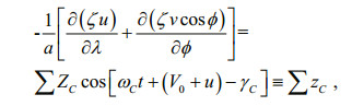
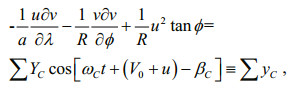
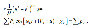
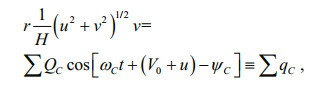
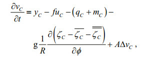
2 NUMERICAL MODEL AND ITS IMPLEMENTATION 2.1 Governing equationsWe use the vertically integrated momentum and continuity equations, inclusive of internal tide dissipation and SAL tide as governing equations. These are written in spherical coordinates as follows.
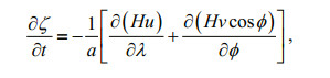 (1)
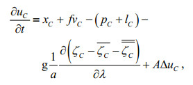
(1)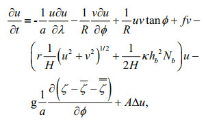 (2)
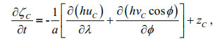
(2)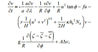 (3)
(3)where u, v are zonal and meridional components of the velocity, t is time, R is the Earth's radius, a=Rcosϕ, λ is longitude, ϕ is latitude, ζ is height of the free surface, ζ and 
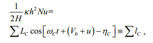
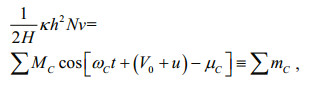
In Eqs. 2 and 3, 
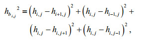 (4)
(4)
Equilibrium tidal heights adjusted for Earth's elasticity are expressed in the form
 (5)
(5)where subscript C stands for the tidal constituent with C=1 for M2 and C=2 for S2, ω is angular speed of the tidal constituents, f is the nodal factor, u is the nodal angle, V0 is initial phase angle, and p=2 for semidiurnal tides. According to Wahr (1981), amplitudes HC for M2 and S2 are equal to the following (in m):

The SAL tide is given as
 (6)
(6)where 
We used the FVCOM, which uses an unstructured grid, for numerical computation. The model domain was 117°-140°E and 18°-41°N. The finest horizontal resolution was 0.04°, as shown in Fig. 2. Along the closed boundary, the normal velocity was set to zero. Along the open boundary, tidal heights were calculated from the harmonic constants of M2 and S2, using
 (7)
(7)

|
| Figure 2 Computation grid |
where HC and GC are harmonic constants obtained from global tidal model DTU10. Harmonic constants of the SAL tides were acquired from Fang et al. (2013) (see Fig.B1 of Appendix for their distribution). The initial condition was ζ=u=v=0 when t=0. The model was run for 30 days, and results of the last 15 days were used for the harmonic analysis.
3 NUMERICAL SIMULATIONIn the numerical simulation, the terms in Eq.6 were all included, and the parameters in the equation were obtained through an optimization procedure.
3.1 Parameter optimizationIn the study area, we selected 59 stations where observed tidal harmonics were available for parameter optimization and model verification. The locations of these stations are shown in Fig. 3. Along the coast of the China mainland, west coast of the Korean Peninsula, and Ryukyu Islands, the harmonic constant was taken from the database of the International Hydrographic Office. For the Taiwan Strait, the harmonic constants were taken from Jan et al. (2002). For the off shore area, the harmonic constants were obtained by analyzing TOPEX/Poseidon altimetry at the crossover points (Wang et al., 2012).

|
| Figure 3 Tidal stations at which tidal harmonic constants were used for parameter optimization and model verification Dots are tidal stations on coasts or islands; crosses are TOPEX/Poseidon crossover points. |
We used the RMS difference between model outputs and observations at 59 stations (Fig. 3) as the cost function to optimize model parameters and evaluate accuracy of the model results. The cost function was calculated by
 (8)
(8)where FC is the RMS vector difference between computed and observed harmonics of the constituent C, taken as
 (9)
(9)where k is the station index, H and G are harmonic constants for amplitude and phase-lag, and Com and Mea are computed and observed results, respectively. The model produces tidal harmonic constants by T_tide (Pawlowicz et al., 2002).
We assumed that the bottom friction and internal tide dissipation coefficients are constants independent of time and space. Based on our previous experience, r was estimated to be ~0.001 5 for the study area, and κ was estimated to be of order of 10-5/m. Thus, the optimal value of r should lie between 0.000 5 and 0.004, and that of κ between 0 and 0.000 1/m. To find the optimal (r, κ) combination, we first performed 48 numerical computations using coarser resolution. Comparing these 48 F values, we found that the minimum F appeared at (r, κ)=(0.001 5, 0.000 02). We took this point as the center, reduced the (r, κ) domain, increased the resolution, and performed a second set of computations. Those showed a minimum F at (r, κ)=(0.001 25, 0.000 03). Finally, we took this new point as the center, further reduced the domain of (r, κ), and executed a third set of computations. From that set, we found that when (r, κ)=(0.001 25, 0.000 035), the value of F was a minimum, 7.71 cm. The third set of computations also revealed no great change among F values at points neighboring that point, indicating that further refined computations were unnecessary. Therefore, we terminated the computation and took (r, κ)=(0.001 25, 0.000 035) as optimal estimates. Results of the three sets of computations are shown in Fig. 4, in which the units of κ are /m. The output obtained with the optimal (r, κ) combination is regarded as the optimal solution. For convenience, the simulation with all terms in Eq.6 included and parameters (r, κ)=(0.001 25, 0.000 035) is called the standard simulation in the following.

|
| Figure 4 Dependence of cost function F on parameter combination (r, κ) |
As stated above, the M2 and S2 mean RMS difference in the standard simulation was 7.71 cm. The mean absolute difference of amplitudes and phase-lags for M2 were 6.36 cm and 5.27° respectively, and those for S2 were 2.66 cm and 5.62°. A detailed station-by-station comparison of model-produced harmonic constants with observations is given in the Appendix.
3.2 Results of standard simulationCotidal charts for M2 and S2 based on the optimal solution are shown in Figs. 5 and 6, respectively. These charts agree well with observed ones from Fang (1986) and Fang et al. (2004), as well as with previous numerical products. This demonstrates that the model with optimized parameters is reliable. Characteristics of the semidiurnal tidal regimes have been ably described in previous works, and so are not repeated in the description here.

|
| Figure 5 Model-produced cotidal chart for M2 constituent Solid line: greenwich phase lag (in degrees); dashed line: amplitude (in cm). |

|
| Figure 6 As in Fig.5, but for S2 |
The energy flux across a section of unit width is called energy flux density (Fang et al., 1999). Vectors of energy flux density for M2 and S2 tides obtained are plotted in Figs. 7 and 8, respectively. These figures clearly show the strongest energy fluxes in passages of the Ryukyu Islands chain. Energy inflow into the East China Sea appears to have three main branches. The north branch is divided into two parts; most energy enters the Yellow Sea circumambulating Cheju Island and extends along the eastern shore, with a very small portion flowing toward the Japan/ East Sea, mainly along the Japanese coast. The middle branch flows northwestward and forms a counterclockwise rotating pattern with a southwest turn along the Shandong Peninsula, then extends southeastward and terminate at the middle North Jiangsu coast. The south branch first flows northward and then turns toward the Taiwan Strait, supporting strong tides there.

|
| Figure 7 Tidal energy flux density vectors of M2 constituent |

|
| Figure 8 Tidal energy flux density vectors of S2 constituent |
To reveal the relative importance of each term in the governing equations, we analyzed the energy balance. The method used was similar to that of Fang et al. (1999). First, the study area was divided into five subareas as shown in Fig. 9. In this figure, G1 through G5 roughly represent the Bohai Sea, Yellow Sea, East China Sea shelf, East China Sea deep basin (including shelf margin and Okinawa Trough), and the east zone of the Ryukyu Islands. Boundaries separating these subareas are marked as B1, B2, B5 and B6. B3 and B4 are open boundaries of G3 connecting the Taiwan Strait and Japan/East Sea, respectively. B7 is the open boundary of G5. G1 to G4 together represent the Bohai, Yellow and East China Seas, the area of focus of the present study. The analysis was conducted constituent by constituent. Because the governing equations contain some nonlinear terms, we first expanded these terms in Fourier forms:
 (10)
(10) (11)
(11) (12)
(12) (13)
(13) (14)
(14) (15)
(15) (16)
(16)

|
| Figure 9 Division of subareas for energy balance analysis |
Because model-produced hourly values of ζ, u and v are available, hourly values of each term on the left sides of the above equations are readily obtained. Then, the amplitudes and phase-lags of these terms (Z and γ in Eq.10) can be derived through harmonic analyses. The number of harmonic terms contained in Eqs.10-16 is larger than that in Eq.7, and we only used terms with frequencies equal to those of M2 and S2. For a specific constituent C, Eqs.1, 2 and 3 become correspondingly
 (17)
(17) (18)
(18) (19)
(19)Multiplying Eqs.17, 18 and 19 by ρgζC, ρguC and ρgvC respectively and adding them, then taking the average for a period, and finally integrating over area G, we obtain
 (20)
(20)where subscript C has been dropped. The four terms on the left side represent energy input, and the three terms on the right side represent energy consumption. The energy flux entering G through its boundary is
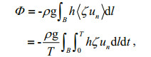 (21)
(21)where T is the period of the constituent; un is the velocity component normal to boundary B and is zero along the closed (solid) boundary, with B representing any of Bi (i=1, 2, …, 7) or their combinations. If Φ is calculated with reference to an area, the outward velocity (or inward flux) component is defi ned as positive. The rate of work done by equilibrium tides on an area G (G representing any of Gi, i=1, 2, …, 5) can be calculated from
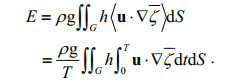 (22)
(22)The rate of work by SAL tides can be calculated by
 (23)
(23)The values of N, Db, Di and Dl are calculated from
 (24)
(24)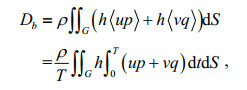 (25)
(25)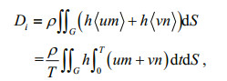 (26)
(26)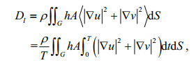 (27)
(27)In comparison with the energy balance equation given by Fang et al. (1999), Eq.20 has two extra terms, i.e., the SAL term S and internal tide dissipation term Di. Because the grid points of FVCOM are irregularly distributed, in practical calculation we first interpolate the model outputs to rectangular grid points, then calculate the integrands in the above equations at these points, finally integrating the integrands over subarea G. The interpolation can induce certain discrepancies, especially near the Ryukyu Islands chain, where islands are numerous and coastlines are very complicated. Thus, calculated values for energy terms in the following cannot completely satisfy the balance required by Eq.20.
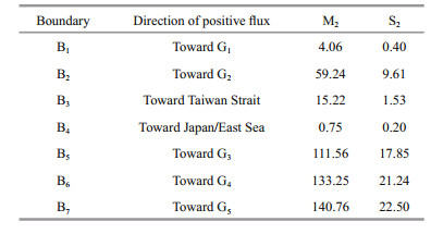
The calculated energy fluxes F through boundaries B1-B7 are listed in Table 1. We see that tides in the Bohai, Yellow, and East China Seas are essentially maintained by energy fluxes from the Pacific Ocean through the Ryukyu Islands passages (B6 in Fig. 9). The magnitudes of the fluxes (133.25 GW for M2; 21.24 GW for S2) agree well with the results of previous studies (see Zhu et al., 2014 and references therein). Energy fluxes through the Taiwan Strait (B3) listed in Table 1 are southwestward and very large, implying strong southwestward semidiurnal waves propagating through the strait. In contrast, northeastward semidiurnal fluxes into the Japan/East Sea (B4) are very small, consistent with weak tides in the sea.
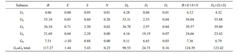
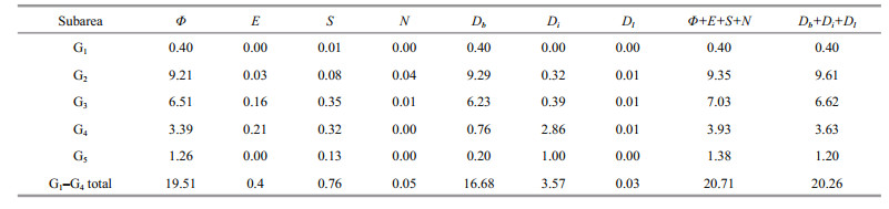
Energy budgets for the five subareas and entire BYECS (G1-G4 total) are shown in Tables 2 and 3 for constituents M2 and S2, respectively. These tables show that maintenance of tidal motion in the study area almost entirely (exceeding 94% for both M2 and S2) relies on the energy flux from outer oceans. The tide-generating force contributes 1.2% M2 power for the entire BYECS and up to 2.8% for the East China Sea deep basin. Strikingly, the SAL tide contributes much more power than the tide-generating force, 4.4% M2 power for the BYECS and up to 9.3% for the East China Sea deep basin. The contribution of the advection term is generally negligible. The total dissipation Db+Di+Dl should be in balance with the total energy input Φ+E+S+N. However, Tables 2 and 3 show a small imbalance, which is mainly caused by model output interpolation, as mentioned above. Among the three dissipation terms, the contribution of lateral friction is very small. Bottom friction plays a major role in dissipating tidal energy in shelf regions G1, G2 and G3. In contrast, the internal tide effect is important in deepwater regions G4 and G5. For the entire BYECS (G1-G4 total in Tables 2 and 3), the bottom friction still dissipates most tidal energy (~80% for both M2 and S2). Total internal tide dissipation for M2 in the entire study area (G1 to G5 together) is estimated at 31 GW, similar to the 35 GW estimate of Niwa and Hibiya (2004) for a larger area. The internal tide dissipation is mostly near the Ryukyu Islands chain, which also agrees with Niwa and Hibiya.
To further demonstrate the influences of the tidegenerating force and SAL tide on the ocean tide in the BYECS, we carried out two additional numerical experiments. In the first (Exp. 1), we artificially removed the tide-generating force in the BYECS (G1 to G4 in Fig. 9) by setting ζ=0 there, and retained the values in G5 as in the standard simulation. The bottom friction, internal parameters and SAL tide were also unchanged. The difference between Exp. 1 and the standard simulation (vector difference of that simulation minus Exp. 1) for M2 is shown in Fig. 10 (S2 is not shown). In the second experiment (Exp. 2), we artificially removed the SAL tide in the BYECS (G1 to G4 in Fig. 9) by setting

|
| Figure 10 Vector difference of standard simulation minus Exp. 1 for M2 Dashed lines indicate amplitude (cm) and solid lines Greenwich phase lag. |

|
| Figure 11 Vector difference of standard simulation minus Exp. 2 for M2 Dashed lines indicate amplitude (cm) and solid lines Greenwich phase lag. |
Figure 10 reveals that the phase-lag distribution of the difference owing to removal of the tide-generating force in BYECS has a certain similarity to that of the cotidal chart (Fig. 5). However, the former lags the latter by ~160° in the southeast, decreasing to ~70° in the northern Yellow Sea, and ~30° in Liaodong Bay. The amplitude reaches its maximum, greater than 30 cm, in the Liaodong Bay. The figure gradually decreases further in Bohai Bay and northeastern North Yellow Sea (>25 cm), to Haizhou Bay (>20 cm) and finally Inchon Bay (~10 cm). Figure 11 shows that the phase-lag distribution of the difference caused by removal of the SAL tide in BYECS is very similar to that of the cotidal chart (Fig. 5). Also, their phase lags have no signifi cant difference. Maximum amplitude (>40 cm) appears in Liaodong Bay. The next largest (>35 cm) was in Bohai Bay, the northeastern North Yellow Sea, and Inchon Bay. Although the amplitude distribution (Fig. 11) of the difference between with and without SAL tide in the forcing term is very similar to that of ocean tide (Fig. 5), the relative magnitude (i.e., role of SAL tide) is spatially variable. For example, in Liaodong Bay, the form for M2 is over 40 cm, amounting to ~1/3 of the latter; whereas in Inchon Bay that form is over 35 cm, only ~1/8 of the latter.
6 SUMMARY AND CONCLUSIONA parameterized internal tide dissipation term and SAL tide term were introduced for the fi rst time in a barotropic numerical model to investigate the dynamics of semidiurnal tidal constituents M2 and S2 in the BYECS. Optimal parameters for bottom friction and internal dissipation were obtained through a series of numerical computations. It was found that:
1. Maintenance of tidal motion in the study area almost entirely (> 94% for both M2 and S2) relies on the energy flux from outer oceans. The tide-generating force contributes 1.2% M2 power for the entire BYECS and up to 2.8% for the East China Sea deep basin. The SAL tide contributes much more power than the tide-generating force, 4.4% M2 power for the BYECS and up to 9.3% for the East China Sea deep basin (including shelf margin and Okinawa Trough);
2. Bottom friction plays a major role in dissipating tidal energy in the shelf regions, and the internal tide eff ect is important in the deepwater regions. For the entire BYECS, the bottom friction dissipates about 80% of tidal energy, and total internal tide dissipation accounts for the remaining 20%, for both M2 and S2;
3. Numerical experiments show that artificial removal of the tide-generating force in the BYECS can cause a signifi cant difference in model output. Maximum magnitude of the difference was in Liaodong Bay, exceeding 30 cm. The artificial removal of SAL tide in the BYECS can cause an even greater difference in model output. The maximum magnitude of the difference was also in Liaodong Bay, exceeding 40 cm. This clearly shows the importance of SAL tide inclusion in the numerical simulation of tides in the waters, even those with a greater proportion of shelf seas.
The main conclusions are as follows: a) internal tide dissipation is important in the shelf margin area and deep waters near the Ryukyu Islands, and can be parameterized by Jayne and St. Laurent's formula; b) the effect of the SAL tide is more important than the tide-generating force for ocean tides in the BYECS, so that tide should be accounted for in numerical simulations, especially if the tide-generating force is considered.
We used the simplest parameterization form for internal tide dissipation, proposed by Jayne and St Laurent (2001). Other forms, such as used by Green and Nycander (2013), should also be used in future tidal modeling of the BYECS. This is especially so for diurnal tides, which were not simulated in the present work.
7 ACKNOWLEDGEMENTWe are grateful to two anonymous reviewers for constructive comments and suggestions on an earlier version of this manuscript.
| Chen C S, Beardsley R C, Cowles G. 2006. An Unstructured Grid, Finite-Volume Coastal Ocean Model: FVCOM User Manual. SMAST/UMASSD. p. 6-8. |
| Choi B H. 1980. A tidal model of the Yellow Sea and the Eastern China Sea. KORDI Report 80-82. Korea Ocean Research and Development Institute. 72p. |
| Egbert G D, Ray R D, 2000. Significant dissipation of tidal energy in the deep ocean inferred from satellite altimeter data. Nature, 405(6788): 775–778. Doi: 10.1038/35015531 |
| Fang G, Kwok Y K, Yu K, et al, 1999. Numerical simulation of principal tidal constituents in the South China Sea, Gulf of Tonkin and Gulf of Thailand. Continental Shelf Research, 19(7): 845–869. Doi: 10.1016/S0278-4343(99)00002-3 |
| Fang G H, Wang Y G, Wei Z X, et al, 2004. Empirical cotidal charts of the Bohai, Yellow, and East China Seas from 10 years of TOPEX/Poseidon altimetry. Journal of Geophysical Research Oceans, 109(C11): C11006. Doi: 10.1029/2004JC002484 |
| Fang G H, Xu X Q, Wei Z X, et al, 2013. Vertical displacement loading tides and self-attraction and loading tides in the Bohai, Yellow, and East China Seas. Science China Earth Sciences, 56(1): 63–70. Doi: 10.1007/s11430-012-4518-9 |
| Fang G H, 1986. Tide and tidal current charts for the marginal seas adjacent to China. Chinese Journal of Oceanology and Limnology, 4(1): 1–16. Doi: 10.1007/BF02850393 |
| Gao X M, Wei Z X, Lü X Q, et al, 2015. Numerical study of tidal dynamics in the South China Sea with adjoint method. Ocean Modelling, 92: 101–114. Doi: 10.1016/j.ocemod.2015.05.010 |
| Green J A M, Nycander J, 2013. A comparison of tidal conversion parameterizations for tidal models. J. Phys.Oceanogr., 43(1): 104–119. Doi: 10.1175/JPO-D-12-023.1 |
| Han G J, Li W, He Z J, et al, 2006. Assimilated tidal results of tide gauge and TOPEX/Poseidon data over the China seas using a variational adjoint approach with a nonlinear numerical model. Advances in Atmospheric Sciences, 23(3): 449–460. Doi: 10.1007/s00376-006-0449-8 |
| Jan S, Chern C S, Wang J, 2002. Transition of tidal waves from the East to South China Seas over the Taiwan Strait:influence of the abrupt step in the topography. Journal of Oceanography, 58(6): 837–850. Doi: 10.1023/A:1022827330693 |
| Jayne S R, St Laurent L C, 2001. Parameterizing tidal dissipation over rough topography. Geophysical Research Letters, 28(5): 811–814. Doi: 10.1029/2000GL012044 |
| Li P L, Zuo J C, Wu D X, et al, 2005. Numerical simulation of semidiurnal constituents in the Bohai Sea, the Yellow Sea and the East China Sea with assimilating TOPEX/Poseidon data. Oceanologia et Limnologia Sinica, 36(1): 24–30. |
| Locarnini R A, Mishonov A V, Antonov J I et al. 2013. World Ocean Atlas 2013, Volume 1: Temperature. NOAA Atlas NESDIS 73, 40p. |
| Lü X Q, Fang G H, 2002. Numerical experiments of the adjoint model for M2 tide in the Bohai Sea. Acta Oceanologica Sinica, 24(1): 17–24. |
| Lü X Q, Zhang J C, 2006. Numerical study on spatially varying bottom friction coefficient of a 2D tidal model with adjoint method. Continental Shelf Research, 26(16): 1 905–1 923. Doi: 10.1016/j.csr.2006.06.007 |
| Niwa Y, Hibiya T. 2004. Three-dimensional numerical simulation of M2 internal tides in the East China Sea. Journal of Geophysical Research, 109(C4): C04027, http://dx.doi.org/10.1029/2003JC001923. |
| Pawlowicz R, Beardsley B, Lentz S, 2002. Classical tidal harmonic analysis including error estimates in MATLAB using T_TIDE. Computers and Geosciences, 28(8): 929–937. Doi: 10.1016/S0098-3004(02)00013-4 |
| Pugh D T. 1987. Tides, Surges and Mean Sea-Level. John Wiley & Sons, Chichester. 471p. |
| Ray R D, 1998. Ocean self-attraction and loading in numerical tidal models. Marine Geodesy, 21(3): 181–192. Doi: 10.1080/01490419809388134 |
| St Laurent L C, Simmons H L, Jayne S R, 2002. Estimating tidally driven mixing in the deep ocean. Geophysical Research Letters, 29(23): 21-1–21-4. Doi: 10.1029/2002GL015633 |
| Wahr J M, 1981. Body tides on an elliptical, rotating, elastic and oceanless earth. Geophys. J. Int., 64(3): 677–703. Doi: 10.1111/gji.1981.64.issue-3 |
| Wang K, Fang G H, Feng S Z, 1999. A 3-D numerical simulation of M2 tides and tidal currents in the Bohai Sea, the Huanghai Sea and the East China Sea. Acta Oceanologica Sinica, 21(4): 1–13. |
| Wang Y H, Fang G H, Wei Z X, et al, 2012. Cotidal charts and tidal power input atlases of the global ocean from TOPEX/Poseidon and JASON-1 altimetry. Acta Oceanologica Sinica, 31(4): 11–23. Doi: 10.1007/s13131-012-0216-x |
| Yanagi T, Morimoto A, Ichikawa K, 1997. Co-tidal and corange charts for the East China Sea and the Yellow Sea derived from satellite altimetric data. Journal of Oceanography, 53: 303–309. |
| Zhao B, Fang G, Cao D, 1993. Numerical modeling on the tides and tidal currents in the Eastern China Sea. Yellow Sea Research, 5: 41–61. |
| Zhu X M, Bao X W, Song D H, et al, 2012. Numerical study on the tides and tidal currents in Bohai Sea, Yellow Sea and East China Sea. Oceanologia et Limnologia Sinica, 43(6): 1 103–1 113. |
| Zhu X M, Song D H, Bao X W, et al, 2014. Tidal energy flux and dissipation in the Northwest Pacific. Journal of Tropical Oceanography, 33(1): 1–9. |
| Zu T T, Gan J P, Erofeeva S Y, 2008. Numerical study of the tide and tidal dynamics in the South China Sea. Deep Sea Research Part Ⅰ:Oceanographic Research Papers, 55(2): 137–154. Doi: 10.1016/j.dsr.2007.10.007 |