 2017, Vol. 35
Institute of Oceanology, Chinese Academy of Sciences
Article Information
- QI Jifeng(齐继峰), YIN Baoshu(尹宝树), ZHANG Qilong(张启龙), YANG Dezhou(杨德周), XU Zhenhua(徐振华)
- Seasonal variation of the Taiwan Warm Current Water and its underlying mechanism
- Chinese Journal of Oceanology and Limnology, 35(5): 1045-1060
- http://dx.doi.org/10.1007/s00343-017-6018-4
Article History
- Received Jan. 18, 2016
- accepted in principle Mar. 24, 2016
- accepted for publication Jul. 8, 2016


2 Key Laboratory of Ocean Circulation and Waves, Chinese Academy of Science, Qingdao 266071, China;
3 Function Laboratory for Ocean Dynamics and Climate, Qingdao National Laboratory for Marine Science and Technology, Qingdao 266000, China;
4 University of Chinese Academy of Science, Beijing 100049, China
The East China Sea (ECS) is located at the western edge of the Pacific Ocean and is well known as a marginal sea with important biological resources. Circulation in this region has been of interest to many researchers because various currents, such as the Kuroshio, the Taiwan Warm Current (TWC), the Taiwan Strait Warm Current (TSWC), the Yellow Sea Warm Current (YSWC), the Cheju Warm Current and the Min-Zhe coastal current (MZCC) flowing southward along Zhejiang-Fujian Province coast (Isobe, 2008) (Fig. 1). The Taiwan Warm Current play an important role in the circulation throughout the ECS (Fang et al., 1991). Therefore, understanding the features of TWC is very critical to understanding the shelf circulation of ECS.

|
| Figure 1 Schematics for the ocean circulation in the Yellow and East China Seas redrawn from Isobe (2008) |
Broken arrows represent ocean currents that are possibly sporadic events in winter. Dotted lines denote depth contour lines of 50 100 and 200 m. A: Kuroshio; B: Taiwan Warm Current; C: Taiwan Strait Warm Current; D: Yellow Sea Warm Current; E: MinZhe Coastal Current; F: Cheju Warm Current.
The Taiwan Warm Current is usually defined to as the currents originating either in the Taiwan Strait or the onshore Kuroshio intrusion northeast of Taiwan Island (Guan and Mao, 1982; Su et al., 1994). It flows northward along the 50-100 m isobaths all year around and transports a great number of warm and saline water into the western ECS shelf region, this warm and saline water composed of the Taiwan Strait water and the Kuroshio water northeast of Taiwan Island is often referred to as the Taiwan Warm Current Water (TWCW) (Weng and Wang, 1984; Zhang and Weng, 1985; Su et al., 1994; Qi et al., 2014; Zhang et al., 2014).
The TWCW is one of the most important water masses in the ECS and has an important impact on the hydrographical conditions and the fishery productions in western ECS shelf area (Liu et al., 1984; Zhang et al., 2007). The cold deep water of TWCW coming from the Kuroshio subsurface waters can provide a major source of nutrients to support primary production in the ECS. For example, Chen (1996) reported that the intruded Kuroshio water can contributes to a great number of nutrients which are many times more than the deposits from the Changjiang (Yangtze) River. It is worth pointing out that the TWCW is often referred to as the Taiwan Warm Current Surface Water (TWCSW), but it separates into the TWCSW and the Taiwan Warm Current Deep Water (TWCDW) during April– September due to the appearance of thermocline (Weng and Wang, 1984). In other words, the TWCW consists of two water masses, i.e., TWCSW and TWCDW in the warm half of the year (April-September), but only one, the TWCSW in the clod half of the year (October-next March). Previous studies indicate that the TWCSW show strong seasonality in its horizontal distribution, T-S characteristics and source. In summer, the TWCSW becomes warmer, fresher and smaller than in winter, and it originates mostly from the Kuroshio Surface Water (KSW) northeast of Taiwan Island and less from the Taiwan Strait water during wintertime, but it consists of the strait water and the KSW during summertime (Zhang et al., 2014).
Although the previous studies achieved several useful result on the TWCW, most of them have mainly focused on the T-S characteristics and spatial distribution of the TWCW and its source in winter and summer, the seasonal variability of its volume has not been well understanding due to the scarcity of long-term observed data. Moreover, the driving mechanisms for seasonal variability of TWCW's volume remain to be unclear until now. In addition, the previous studies are mostly obtained based on the data observed in a synoptic voyage (which can be referred to as a weather analysis), while it is very rare to study the TWCW (or TWCSW) with the climatological monthly data (This can be referred to as a climatological analysis). As everyone knows, the distribution and T-S characteristics of TWCW depend largely on the weather and other external factors (such as typhoon and mesoscale eddies), and once these external factors appear mutation, then the TWCW will undergo great changes in its distribution and T-S features (Li and Su, 2000; Zhang et al., 2014). Although the weather analysis results are of distinguishing features, they also have their limitations, for these results cannot fully reflect the climatic characteristics of the TWCW. So, a comprehensive understanding of seasonality of the TWCW is still an important goal.
In this study, we clarify quantitatively the seasonal variation of the TWCW (such as T-S properties, spatial distribution and volume) based on the climatological monthly T and S data obtained from the U.S. National Oceanic Data Center (NODC) and the Institute of Oceanology, Chinese Academy of Sciences, China, and examine the underlying dynamic factors controlling the seasonal variation of the TWCW by using the modeling results. The remaining of the paper is organized as follows. Section 2 briefly describes the observed dataset and the analysis method used in this study. The seasonal variation of the TWCW is discussed in Section 3. Section 4 mainly examines the driving mechanisms for the seasonal variation in the TWCW. The paper ends with conclusions in Section 5.
2 DATA AND METHODOLOGY 2.1 Data and validationsThe historical T and S data used in the present study were selected from the Ocean Science Database, Institute of Oceanology, Chinese Academy of sciences (OSD-IOCAS) (Wang et al., 2004), which collected hydrographic observation data from 1930 through 2001 from various Chinses marine hydrological surveys and international data sets, including the World Ocean Database 2013 (WOD13). The WOD13 data can be obtained from the U.S. National Oceanic Data Center (NODC), which include ocean station data (Nansen bottle), conductivity-temperature-depth (CTD), mechanical bathythermograph (MBT), and expandable bathythermograph (XBT) data, cover more coastal regions compared with the WOD09. The primary quality control of these data follows the methods outlined by Boyer and Levitus (1994). Further quality control methods were developed and applied to prevent repeated, wrong, or manmade data from entering the database (Wang et al., 2004). Several steps of the quality control procedure were carried out, including inspections and eliminations of duplicate profiles, inversed and duplicated depths and densities in individual profiles, and statistical based criterion ranges of parameter varying with depth, season, and location.
In the vertical direction, all data were interpolated by a piecewise cubic spline method to obtain 5 m vertical resolution. In the horizontal direction, data at each level were gridded on a grid of 0.5°×0.5° through an objective interpolation scheme, and only the cells including more than 3 points were retained for further analysis. The missing data can be filled by use of a weighted average of four neighboring grid point values. In order to describe the distribution of the bottom water masses, we chose the depth of 200 m to be representative of depths greater than 200 m.
Numerical simulation result from our fineresolution model is also used to examine the possible causes for the seasonal variation in the TWCW. Considering the important influence of the Changjiang River on the distribution of the water masses in the ECS, our ROMS set up includes the Changjiang River discharge. The study area (a dashed line box) is shown in Fig. 2.

|
| Figure 2 The model domain and bathymetry of study area, and locations of station (black spots) Contour lines represent isobaths and numbers indicate depth. Abbreviations are used for the East Taiwan Channel (ETC), and Tsushima Strait (TS), respectively. |
To check the accuracy of the model data, the model results are compared with observations in terms of both velocity field and volume transport. Figures 3 and 4 show the simulated monthly mean surface and bottom velocity field in the southwestern ECS in different seasons. The current system in the study area, which consists of Kuroshio, TWC and MZCC, is well reproduced. The Kuroshio northeast of Taiwan Island is matches well the long-term observation data (Qiu and Imasato, 1990, Fig. 3). Furthermore, the seasonal variation of these current is well reproduced by our model. i.e., the MZCC has been observed in winter, but it is obscure in summer. In summer, the TWC is mainly coming from the Taiwan Strait. However, in winter, it comes mainly from the shelf intrusion of the Kuroshio northeast of Taiwan Island. These features of current system are consistent with observations (Isobe, 2008). Furthermore, we compared monthly mean volume transport across the Tsushima Strait (TS) and the East Taiwan Channel (ETC) with observations, where long-term continuous observations have been conducted (Fig. 2). The Kuroshio transport through the ETC, as shown in Fig. 5b, is calculated with the direct method of Johns et al. (2001) using ADCP and current meter measurements. It is seen that both the simulated and observed volume transport across TS and ETC are in good agreement in both magnitude and phase (Fig. 5). The simulated transport were of the same order as those reported by previous studies (Johns et al., 2001; Takikawa et al., 2005; Isobe, 2008). As discussed above, our model results agree well with the observations. More detailed model configuration and examination of the model results can be found in our earlier publication (Yang et al., 2011).

|
| Figure 3 Monthly mean surface current fields in (a) February, (b) May, (c) August, and (d) November |

|
| Figure 4 Monthly mean bottom current fields in (a) February, (b) May, (c) August, and (d) November |

|
| Figure 5 Comparison of modeled and observed results a. volume transport through the Tsushima Strait (redrawn from Takikawa et al., 2005 and Isobe, 2008); b. volume transport through the PCM section. |
In order to study the distribution and variation of the TWCW, it is necessary to determine the range of the TWCW accurately. The conventional method is the cluster analysis method, which enables objects of similar kinds to be grouped into respective categories from massive data such as CTD data (Li and Su, 2000). The procedure begins by making each data point a single cluster, which is, given n data points, n clusters exist. In every iterations, the closest two clusters are combined into a new cluster until the total cluster number reaches a designated level. The decision as to which clusters to combine is based on the distance functions (FD). Thus, once a distance function (FD) is specified, the analysis becomes objective because there is no subjective factors to determine the function. So, the definition of FD is very important. Previous studies suggested that the temperature and salinity are two important indexes of water mass characteristics, and the station points with similar T-S properties should be divided into the same cluster. In addition, it was further pointed out that the depth and geographical distance of the sample should also be included in distance function (Hur et al., 1999). Although T-S diagrams have been also used to study the water masses in the China Seas, they are not as objective as the cluster analysis method and cannot define the water masses accurately. So, a distance function including several important variables (temperature, salinity, depth, and geographical distance) are applied to identify the hydrographic features of the TWCW.
Before analysis begins, normalization of each variable for each of the methods is essential due to the differences in units and variable range. In this paper, all T, S and depth data were normalized as follows:
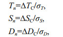
where ∆TC, ∆SC and DC are the T, S and depth distances between two clusters, and ∆σT, ∆σS and ∆σD stand for the standard deviations of T, S and depth in the dataset, respectively. The distance function can be defined by FD=Tn2+Sn2+Dn2+L/LC, where L and LC are the geographic distance and a characteristic distance scale, respectively. LC is a constant with a value of 20 km, which means that this distance contributes to one standard deviation of FD. This definition is similar to that of Hur et al. (1999). In this study, the contribution of temperature, salinity and depth to the distance function is based on the average-linkage. The single-linkage method is used for geographical distance. That is, the geographic distance between the closest two points of two clusters is used for the distance function (Wilks, 1995). Considering that the Changjiang River diluted water is characterized by low salinity, we treat those of the salinity less than 28.00 as the Continental Coastal Water (CCW) before calculating, which is excluded throughout the cluster analysis. Because the TWCW has very similar T-S characteristics to the intruded Kuroshio water along the continental shelf of ECS, it is difficult to define its eastern boundary south of 28°N. Thus, we chose the 200 m isobaths as TWCW eastern boundary position south of 28°N. From a quantitative perspective, this is reasonable. In order to calculate the volume of TWCW, each standard level was analyzed by the analysis method. Combining clustering method with T-S diagrams, we obtained the volume of TWCW in different months. In this paper, we discuss the seasonal variation of the TWCW, and the spring, summer, autumn and winter case are represented by the results of May, August, November, and February, respectively.
3 SEASONAL VARIATION IN TWCWBefore the cluster analysis, the T-S diagrams of the gridded data in summer (August) and winter (February) are depicted in Fig. 6, respectively. Typical T-S diagrams demonstrated that there are three fundamental water masses in the study area during wintertime, i.e., water mass (A) is cold (8.1-16.5℃) and fresh water (less than 32), water mass (B) is cold (9-13.5℃) and relative saline (32.2-33.75) water, water mass (C) is warm (12.3-21.8℃) and saline (33.5-34.6) water, while there are four water masses during summertime, i.e., A, B, C and D which is a cold and saline water. In terms of T-S features, water mass (A) is similar to the Continental Coastal Water (CCW) (Qi et al., 2014), water mass (B) to the YellowEast China Sea Mixing Water (YEMW) (Li and Su 2000), water mass (C) to the Taiwan Warm Current Surface Water (TWCSW), and water mass (D) to the Taiwan Warm Current Deep Water (TWCDW) (Weng and Wang, 1985).

|
| Figure 6 T-S diagrams in the continental shelf of ECS in February and August The points with salinity less than 28.00 were excluded in this diagram. |
Therefore, based on only the T-S distributions there are three water masses which consist of CCW, YEMW and TWCSW in winter. However, summer water mass distribution becomes relatively complex due to increasing intensity of the surface heating, Changjiang River discharge and rainfall. This complicates the task of subjectively distinguishing different summer water masses based on only the T-S distributions. We can't obtain the range of the TWCW accurately by using T-S diagrams. Therefore, the cluster analysis is strong seasonal variability of the water properties in the study area. The point at which to stop iterating is defined as 6 clusters based on the consideration of the number of water masses that prior studies defined in the area (3-6). However, several of the final 6 clusters for each month contain only a few data points. Only cluster which are composed of a significant number of data points (8 or more) are displayed and discussed in the results.
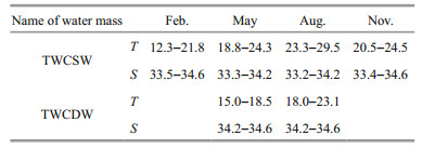
The results of the cluster analysis distinguish the four major water masses: CCW, YEMW and TWCW (which splits into TWCSW and TWCDW during warm half of the year) (Figs. 7 and 8). The CCW is formed by the mixing of seawater with runoff from the Changjiang River, Minjiang River and other rivers. The results indicate that the CCW is located mainly in the coastal area of the western ECS. It exists throughout the year and show seasonal variation in both its extent and T-S properties. In winter (February), the CCW is distributed on the inner continental shelf in a belt shape, and its southern boundary can reach its southern most location of 24°N (25°N) in the surface (bottom) layer. This water mass is coldest with a temperature range of 7.0-15.5℃ and most salty with a salinity range of 30.4-32.2 in winter (not shown). In summer (August), the CCW reaches its easternmost location of 126°E, and the south edge reaches its northernmost location of 27°N. It is warmest with a temperature range of 22.0-28.0℃ and freshest with a salinity range of 27.0-31.0 in this time. Figures 7 and 8 show that the YEMW also show strong seasonal variation in its spatial distribution. In winter its southern edge reaching near 31°N, but it retreats to the Yellow Sea due to the abnormal eastward expansion of the Changjiang River Diluted Water in summer. Its temperature is highest in summer (18.3-22.4℃) and lowest in winter (7.5-13.5℃), but the reverse is true for salinity; the salinity is lowest (31.5-32.4) in summer and highest (32.5-33.6) in winter (not shown). Since the main objective of this paper is to study the seasonal variation of the TWCW, we won't discuss above two water masses further in this paper. Next, we mainly discuss the seasonal variation of the TWCW. The results indicate that the TWCW consists of the TWCSW and the TWCDW during the warm half of the year but only the TWCSW during the cold half of the year (October to next March). The T-S characteristics of the TWCW are shown in Table 1. In addition, according to the spatial range of the TWCSW and TWCDW at each level in four seasons, we calculated the volumes of the TWCW in every month, the results are shown in Table 2.

|
| Figure 7 Horizontal distributions of water masses at the surface layer in (a) February, (b) May, (c) August, and (d) November |


|
| Figure 8 Horizontal distributions of water masses at the bottom layer in (a) February, (b) May, (c) August, and (d) November |
In winter (February), the TWCW only consists of the TWCSW due to the disappearance of the thermocline. As shown in Figs. 7 and 8, the TWCSW is mainly distributed in the whole water volume from surface to bottom layer, but its horizontal distribution is larger at the surface layer than at the bottom layer, whose northern boundary could reach to 31.0°N at the surface layer but only to 30.0°N at the bottom layer. Thus, the TWCSW has a volume of 13 746 km3, occupying 41.0% of the whole study area (25°-32°N, 119°-126°E). Meanwhile, the TWCSW is coldest with a temperature range of 12.3-21.8℃ and most salty with a salinity range of 33.5-34.6 in a year due to low sea surface heat fluxes, less precipitation and strong vertical mixing of sea water.
3.2 In springIn spring (May), due to the appearance of thermocline under the combined actions of the weak vertical mixing and surface heating, the TWCDW has formed and is distributed in the deep layer below the TWCSW, and thus the TWCW is composed of two water masses, TWCSW and TWCDW (as shown in Fig. 9a). The spatial range of the TWCSW is smaller at the surface layer than that in winter, mainly due to its north boundary only reaching about 30.0°N, although its western boundary extends somewhat farther to the west than that in winter. Therefore, the TWCSW has a smaller volume with a value of 12 553 km3 than that in winter, occupying 37.4% of the whole study area. Moreover, the TWCSW becomes warmer with a temperature range of 18.8-24.3℃ and fresher with a salinity range of 33.3-34.2.

|
| Figure 9 Schematic diagram of the spatial distribution of the water masses in the ECS (a) and the location of transects (b) |
Comparing with TWCSW, the TWCDW has a smaller range and volume (only 4 185 km3) than the TWCSW does. It is worth pointing out that the TWCDW is characterized by low temperature and high salinity, and its temperature and salinity ranges are 15.0-18.5℃ and 34.2-34.6, respectively.
3.3 In summerIn summer (August), the TWCW still consists of the TWCSW and the TWCDW, whose distributions are obviously different from that in spring. The TWCSW weakens in its northward-extension (The northern boundary reaches only about 29.5°N), but strengthens in its westward-extension (the western boundary can reach the vicinity of 119.5°E). Thus, it has a smaller volume (8 289 km3) than in spring. Meanwhile, the TWCSW is much warmer with a temperature range of 23.3-29.5℃ and fresher with a salinity range of 33.2-34.2 than in spring.
Unlike the TWCSW, the TWCDW strengthens in its northward extension (the north boundary can reach about 31.3°N) and in its westward extension (the western boundary can reach about 121.5°E). Therefore, the TWCDW becomes lager with a volume of 4 876 km3, and warmer with a temperature range of 18.0-23.1℃, but its salinity is the same as that in spring.
3.4 In autumnIn autumn (November), under the combined actions of the stronger vertical mixing and surface cooling, the vertical thermohaline structure becomes uniform in the study area and the TWCDW disappears again. Thus, the TWCW only consists of the TWCSW. As shown in Figs. 7 and 8, the TWCSW is distributed in the whole water volume from surface to bottom and has a larger coverage in the surface layer than that in the bottom layer, whose north boundary can reach to 30.3°N and west edge reaches only to the vicinity of 121.0°E in the surface layer. However, the TWCSW is smaller in the deeper layer than that in the surface layer, for its northern boundary reaches only about 29.5°N. Therefore, the TWCW has a volume of 11 397 km3 smaller than in summer, occupying 34.0% of the whole study area. Meanwhile, it becomes colder with a temperature range of 20.5-24.5℃ and more salty with a salinity range of 33.4-34.6.
As mentioned above, the TWCW shows a strong seasonal variability in its volume and T-S properties. If the sum of the TWCSW and TWCDW volumes is regarded as the volume of the TWCW, the annual range of the volume is 11 397-13 746 km3 with some fluctuations as shown in Table 2. The volume of the TWCW increase gradually from November to February and reach a maximum of 13 746 km3 in February. After that, it decrease gradually until May with a second minimum value of 12 553 km3. In summer, the volume of the TWCW increases again with a second maximum value of 13 165 km3 in August. In autumn, it decrease rapidly and reach a minimum of 11 397 km3 in November. What are the causes responsible for the seasonal variation of the volume of TWCW? Next, we discussed this issue in detail.
4 DRIVING MECHANISM FOR SEASONAL VARIATION IN TWCWAs discussed above, the TWCW is mainly composed of the Taiwan Strait water and the Kuroshio waters (KSW and KSSW) (Weng and Wang, 1985; Zhang et al., 2014; Chen et al., 2016). This implies that the TWCW is significantly influenced by the Kuroshio and the TSWC. So, it is necessary to examine the combined effects of Kuroshio and TSWC on the TWCW volume on seasonal time scales. Due to the lack of observed current data, we used the model current data simulated by ROMS (Regional Ocean Modeling System) to examine quantitatively the contributions of the TSCW and Kuroshio water to the TWCW, respectively. To quantitatively clarify the contributions of the TSCW to the TWCW, we have calculated the volume transport of the TSCW through the northern Taiwan Strait (Transect 2 in Fig. 9b) and the TWCW through Section 28°N (Transect 1 in Fig. 9b) in each months, respectively. Table 3 shows the calculated results all year round.
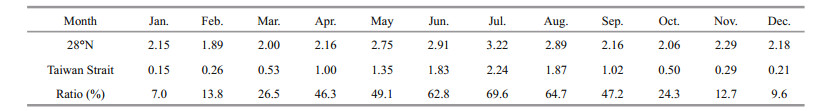 |
During winter, the northerly wind prevails over the study area (Fig. 10a), the evaporation is strongly intensified, but both the net heat flux and precipitation decrease rapidly (not shown). As a result, the vertical thermohaline structure of water volume seems to be uniform from surface to bottom (Li and Su, 2000; Hao et al., 2012). Thus, the TWCW is only composed of the TWCSW due to the disappearance of the TWCDW, but it has a maximum volume. As shown in Figs. 3 and 4, the TSWC becomes weak under the influence of the strong northerly winds, and its volume transport through the northern Taiwan Strait is 0.26 Sv with a transport ratio of 13.8% of the TSWC to the TWCW through Section 28°N. This means that the TSWC makes very small contributions to the TWCW in winter, similar to the previous studies (Zhang et al., 2014). In spring, however, the sea temperature increases gradually due to the sea surface heating and the weaker vertical mixing, and thus the thermoclines begin to form in the study area. At this period, although the TWCDW appears and is distributed in the deep layer, the TWCW begins to become small due to the remarkably small TWCSW. During spring, although the northeasterly winds prevail over the study area, the TSWC begins to strengthen in the surface layer (Fig. 3b), and its volume transport through the northern Taiwan Strait is 1.35 Sv with a transport ratio of 49.1% of the TSWC to the TWCW through Section 28°N, which may provide more strait water for the TWCSW. This indicated that the TSWC could make greater contributions to the TWCW in spring than that in winter. In summer, on the contrary, the strong southerly winds control the study area, and the thermocline (halocline) reach their maximum in the ECS shelf region due to the rapid increase of the net heat flux and precipitation. At this period, the TSCW has strengthened under the influence of the strong southerly winds (Figs. 3c and 4c), and thus its volume transport reaches 1.87 Sv through the northern Taiwan Strait with a transport ratio of 64.7%, which may transport much more strait water to the TWCSW, and the TWCW becomes larger than in spring. Obviously, the TSWC makes greatest contributions to the TWCW in summer. In autumn, the thermocline disappears due to the surface cooling, lower precipitation and stronger vertical mixing in the study area. Therefore, the TWCW is only composed of the TWCSW due to the disappearance of the TWCDW, similar to the condition in winter. Driven by the northeasterly winds over the study area, the TSWC becomes weaker again, and its volume transport through the northern Taiwan Strait is 0.29 Sv with a transport ratio of 12.7%, suggesting that the TSWC makes much smaller contributions to the TWCW than in summer.

|
| Figure 10 Monthly climatological wind-stress fields in (a) February, (b) May, (c) August, and (d) November (unit: N/m2) from COADS (Kent et al., 2007) |
It should be pointed out that the contributions of the TSWC to the TWCW are greatest (69.6%) in July, secondary (64.7% and 62.8%) in August and June (Table 3), and small in the cold half of the year.
The current and seawater volume transport through the Taiwan Strait have been studied by some previous studies, who suggested that the TSWC shows strong variability due to its special geographical position where dynamic processes are dominated by the monsoons, inter-basin pressure and bottom topography (Chuang, 1986; Fang et al., 1991; Jan et al., 2002; Wang et al., 2003; Bai and Hu, 2004; Guo et al., 2005; Hu et al., 2010; Zhu et al., 2015; Chen et al., 2016). As a typical early understanding of the currents in the Taiwan Strait, the monsoon system can influence the flow variations around Taiwan Island (Nitani, 1972). To further clarify the correlations between TSWC and local winds anomalies, based on our modeling results, we have calculated the monthly anomaly of the volume transport through Taiwan Strait, and the monthly anomaly of the along-strait wind stress over the Taiwan Strait. The results are shown in Fig. 11.

|
| Figure 11 Monthly anomaly of the volume transport through Taiwan Strait and the along-strait wind stress over the Taiwan Strait |
As shown in Fig. 11, the seasonal variation of the volume transport through Taiwan Strait is generally consistent with the seasonal variation of the local along-strait winds. Both of them are virtually in phase with each other and display similar variation trends. From January to July, both the monthly anomaly of volume transport and along-strait wind stress increase gradually and reach their maximum in July, and then both of them begin to decrease gradually until reach their minimum from November to December. Obviously, the volume transport through Taiwan Strait varies largely with the local monsoon winds. The high correlation between alongstrait wind and volume transport suggest that the local monsoon winds is the major factor influencing the volume transport through the Taiwan Strait, which control the contribution of the TSWC to the TWCW significantly.
4.2 Contribution of the Kuroshio onshore intrusion northeast of Taiwan Island to TWCWIn winter, under the influence of the strong northerly winds (Fig. 10a), the onshore intrusion of the Kuroshio and the southward coastal currents are both very strong, but the TSWC is considerably weak (Figs. 3a and 4a), the strong Kuroshio onshore intrusion could provide a large amount of the KSW for the TWCW due to the disappearance of the KSSW in the cold half of the year. This indicated that the onshore Kuroshio intrusion northeast of Taiwan Island makes extremely great contributions to the TWCW in winter. In spring, however, the Kuroshio exhibits relative weaker onshore intrusion northeast of Taiwan Island than in winter, but the TSWC begins to strengthen in the surface layer (Fig. 3b). At the same time, the KSSW is separated from the KSW due to the appearance of the thermocline and becomes an independent water mass. Because the TWCW is composed of the TWCSW and TWCDW in this season, the TSWC transports a part of strait water to the TWCSW, and the Kuroshio simultaneously carries a part of KSW into the TWCSW, while the Kuroshio also transports a part of KSSW to the TWCDW. From the volume transport ratio (49.1%) of the TSWC to the TWCW through Section 28°N, we inferred that the Kuroshio onshore intrusion could make similar contributions to the TWCW as the TSWC does in spring. In summer, as shown in Figs. 3c and 4c, the Kuroshio has a weaker shelf-intrusion than in spring, while the TSWC is strongest driven by the strong southerly winds. Because the KSW and the KSSW still exit in summer, the Kuroshio intrudes onto the ECS shelf and provides a part of KSW for the TWCSW and a part of KSSW for the TWCDW, respectively. From the volume transport ratio (69.6%) of the TSWC to the TWCW through Section 28°N in July, we concluded that the TSWC could make greater contributions to the TWCW than the Kuroshio onshore intrusion in summer. In autumn, however, the Kuroshio onshore intrusion begins to strengthen again, and the KSSW is merged into the KSW due to the disappearance of thermocline. As mentioned above, the TSWC is weaker and has a very lower volume transport with 0.29 Sv. Thus, we believed that the Kuroshio onshore intrusion makes much greater contributions to the TWCW than the TSWC in autumn.
As discussed above, the Kuroshio onshore intrusion makes greater contributions to the TWCW than the TSWC except in summer months (June to August). Next, we discuss the driving mechanism controlling the seasonal variation of the Kuroshio onshore intrusion. Located along the pathway of the East Asian monsoon system, the circulation in the study area region is largely influenced by the seasonal reversal of the monsoonal winds from northeasterly in winter to southwesterly in summer (Isobe, 1999; Guo et al., 2006). To illustrate the impacts of winds on contribution of the Kuroshio onshore intrusion to TWCW, based on the Ekman dynamic theory, we calculated the Ekman transport across the Transect 3 in the study area (Fig. 9b), which is a part of total Kuroshio onshore flux. The results are shown in Fig. 12a.

|
| Figure 12 Monthly Kuroshio onshore flux across 200 m isobaths, monthly Ekman transport across the 200 m isobaths, monthly Kuroshio onshore flux across 0–60 m and monthly Kuroshio onshore flux across 60 m to bottom (a); monthly value of the six terms in Eq.1, in which WSE denotes wind stress Ekman term, WSP the wind stress pumping term, BS the bottom stress term, DIF the horizontal diffusion term, and ADV the advection term (b) |
As revealed in Fig. 12a, the Ekman transport shows strong seasonality with a maximum (0.67 Sv) in December and minimum (-0.26 Sv) in July. In order to specify the Kuroshio intrusion, we also calculated the quantitative value of the total Kuroshio onshore flux through the local sections. The depth of the Ekman layer in the shelf break region of ECS is less than 60 m, hence, we divided the 200 m isobaths fluxes into two layers: the surface layer (0-60 m) and the deep layer (60 m to bottom), and the annual cycles in calculated volume transport each layer are shown in Fig. 12a. The volume transport in the surface layer contributes more than 54.4% of the mean Kuroshio onshore flux and has a strong seasonal variation, but the transport in the deep layer has a weaker seasonal variation and contributes less to the Kuroshio onshore intrusion throughout the year. Moreover, the variation tendency of the Ekman transport also corresponds well to that of the surface layer flux, and they show a strong seasonal variation with a minimum in July and a maximum in December.
As seen in Fig. 12a, the annual averaged Kuroshio onshore flux (1.48 Sv) is primarily balanced by the surface layer onshore flux (0.80 Sv), while the deep layer onshore flux plays a secondary role in this variation. Comparing with the deep layer flux, the seasonal variation of the surface onshore flux is generally consistent with the total Kuroshio onshore intrusion flux, which is primarily balanced by the surface Ekman transport induced by the monsoon winds. This indicated that the monsoon winds may be the major factor controlling the contribution of the Kuroshio to the TWCW.
However, the Kuroshio is a complex current system, its variation must be the result of concurrent effects of various factors and mechanism. So, besides the local monsoon winds, there must be other factors influencing the change of the Kuroshio onshore intrusion. To further investigate this problem in more detail, we adopted a traditional method usually used by the previous studies, which can separate the contribution of local wind to transport from that of other factors to examine the effect of the other factors on the seasonal variation of the Kuroshio onshore flux (Mertz and Wright, 1992; Guo et al., 2006).
The methods is carried as follows, firstly, we start from the primitive equations. After vertically averaging the momentum equations and then taking a curl, we get the following vorticity equation (for detailed derivation, see Appendix A):
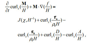 (1)
(1)In Eq.1, two operators are defined as 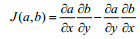
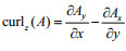
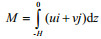

It should be pointed out that the first term in the left-hand side of Eq.1 is negligible in a quasi-steady state such as monthly mean state; hence, the second term M•▽(f/H) [hereinafter referred to as APV (advection of the geostrophic potential vorticity)] is balanced by the five terms in the right-hand side of Eq.1. A positive APV means an onshore intrusion of Kuroshio in the shelf break of ECS.
The monthly APV as well as the other five terms in the equation are integrated along the 200 m isobaths in the study area. It should be noted that the wind stress term can be divided into two terms: the surface Ekman flux (Ekman term about 93%) and the Ekman pumping (Pumping term about 7%) (Isobe, 1999). As shown in Fig. 12b, the wind stress term (WSE) shows a pattern similar to that of APV, which means that the seasonal variation of APV is mainly due to the wind stress term. This result is consistent with the results of previous studies (e.g., Guo et al., 2006). In addition, comparing with the bottom stress term, the horizontal diffusion term and the advection term, the JEBAR term also exhibit a relative stronger seasonal variation, which gradually increase from April to December, and decrease to the minimum in April. On the other hand, the seasonality of the Kuroshio onshore flux is primarily balanced by the wind stress term and the JEBAR term is secondary. The causes for the change of JEBAR term, Oey et al. (2010) demonstrated that the joint effect of baroclinicity and relief (JEBAR) is mainly related to the surface heat flux gradient over the ECS shelf. This means that the surface heat flux is another important factor and play a secondary role in controlling the seasonal variation of the Kuroshio onshore flux. All other terms are less essential to the seasonal variation of the Kuroshio onshore flux since these terms have weaker seasonal change. The analysis in this subsection demonstrate that the wind-induced surface Ekman transport along the 200 m isobaths northeast of Taiwan Island and the change of the surface heat flux are probably two dynamic factors controlling the contribution of the Kuroshio to the TWCW. The comparison demonstrated that the seasonal variation of the total onshore Kuroshio intrusion across the 200 m isobaths is mainly dominated by the local monsoon winds, but its dependence on the wind is obviously modified by the surface heat flux (which induces the change in the density field).
5 CONCLUSIONBased on the historical observed data and the modeling results, this paper investigated the seasonal variation of the TWCW using a cluster analysis method and discussed the contributions of the Kuroshio onshore intrusion and the TSWC to the TWCW volume on seasonal scales. The TWCW has a strong seasonal variation in its horizontal distribution, T-S characteristics and volume. This water mass consists of only the TWCSW in the cold half of the year (October to next March), but of both the TWCSW and the TWCDW in the warm half of the year (April to September). The TWCW is characterized by high (low) temperature and low (high) salinity in summer (winter), whereas its volume is maximum (13 746 km3) in winter and minimum (11 397 km3) in autumn.
The two major sources of the TWCW are the water coming from the TSWC and the Kuroshio intrusion. The TSWC displays strong seasonal variability being strongest (2.24 Sv) in July and weakest (0.15 Sv) in January, its contributions to the TWCW are greatest (69.6%) in July and smallest (7.0%) in January. The onshore Kuroshio intrusion makes greater contributions to the TWCW than the TSWC in most months of a year except in summer months (June to August), when the TSWC makes greater contributions than the onshore Kuroshio intrusion. Diagnostic analysis suggest that the TSWC and the onshore Kuroshio intrusion are controlled by the local monsoon winds on the seasonal scales, the local winds is the dominant factor controlling the seasonal variability in the TWCW volume, while the surface heat flux can play a secondary role via the joint effect of baroclinicity and relief.
6 ACKNOWLEDGMENTThe authors thank Prof. WANG Fan for providing OSD-IOCAS data.
| Bai X Z, Hu D X, 2004. A numerical study on seasonal variations of the Taiwan Warm Current. Chinese Journal of Oceanology and Limnology, 22(3): 278–285. Doi: 10.1007/BF02842560 |
| Boyer T, Levitus S. 1994. Quality control and processing of historical oceanographic temperature, salinity, and oxygen data. NOAA Technical Report NESDIS 81. National Oceanographic Data Center, Washington D. C. |
| Chen C T A, 1996. The Kuroshio intermediate water is the major source of nutrients on the East China Sea continental shelf. Oceanologica Acta, 19(5): 523–527. |
| Chen H W, Liu C T, Matsuno T, et al, 2016. Temporal variations of volume transport through the Taiwan Strait, as identified by three-year measurements. Continental Shelf Research, 114: 41–53. Doi: 10.1016/j.csr.2015.12.010 |
| Chuang W S, 1986. A note on the driving mechanisms of current in the Taiwan Strait. Journal of Oceanography, 42(5): 355–361. Doi: 10.1007/BF02110430 |
| Fang G H, Zhao B R, Zhu Y H, 1991. Water volume transport through the Taiwan Strait and the continental shelf of the East China Sea measured with current meters. Elsevier Oceanography Series, 54: 345–358. Doi: 10.1016/S0422-9894(08)70107-7 |
| Guan B X, Mao H L, 1982. A note on circulation of the East China Sea. Chinese Journal of Oceanology and Limnology, 1(1): 5–16. Doi: 10.1007/BF02852887 |
| Guo J S, Hu X M, Yuan Y L, 2005. A diagnostic analysis of variations in volume transport through the Taiwan Strait using satellite altimeter data. Advances in Marine Science, 23(1): 20–26. |
| Guo X Y, Miyazawa Y, Yamagata T, 2006. The Kuroshio onshore intrusion along the shelf break of the East China Sea:the origin of the Tsushima warm current. Journal of Physical Oceanography, 36(12): 2 205–2 231. Doi: 10.1175/JPO2976.1 |
| Hao J J, Chen Y L, Wang F, Lin P F. 2012. Seasonal thermocline in the China Seas and northwestern Pacific Ocean. Journal of Geophysical Research, 117(C2), http://dx.doi.org/10.1029/2011JC007246. |
| Hu J Y, Kawamura H, Li C Y, et al, 2010. Review on current and seawater volume transport through the Taiwan Strait. Journal of Oceanography, 66(5): 591–610. Doi: 10.1007/s10872-010-0049-1 |
| Hur H B, Jacobs G A, Teague W J, 1999. Monthly variations of water masses in the Yellow and East China Seas, November 6, 1998. Journal of Oceanography, 55(2): 171–184. Doi: 10.1023/A:1007885828278 |
| Isobe A, 1999. On the origin of the Tsushima Warm Current and its seasonality. Continental Shelf Research, 19(1): 117–133. Doi: 10.1016/S0278-4343(98)00065-X |
| Isobe A, 2008. Recent advances in ocean-circulation research on the Yellow Sea and East China Sea shelves. Journal of Oceanography, 64(4): 569–584. Doi: 10.1007/s10872-008-0048-7 |
| Jan S, Wang J, Chern C S, Chao S Y, 2002. Seasonal variation of the circulation in the Taiwan Strait. Journal of Marine Systems, 35(3-4): 249–268. Doi: 10.1016/S0924-7963(02)00130-6 |
| Johns W E, Lee T N, Zhang D X, et al, 2001. The Kuroshio east of Taiwan:Moored transport observations from the WOCE PCM-1 array. Journal of Physical Oceanography, 31(4): 1 031–1 053. Doi: 10.1175/1520-0485(2001)031<1031:TKEOTM>2.0.CO;2 |
| Kent E, Woodruff S, Rayner N, et al, 2007. Advances in the use of historical marine climate data. Bulletin of the American Meteorological Society, 88(4): 559–564. Doi: 10.1175/BAMS-88-4-559 |
| Li F Q, Su Y S. 2000. Analyzing of Oceanic Water Masses. Ocean University of Qingdao Press, Qingdao. 344p. |
| Liu S X, Han S X, Wei Y K, 1984. Analysis of water-masses of north-western Donghai Sea and their relations to fishing grounds. Journal of Fisheries of China, 8(2): 125–133. |
| Mertz G, Wright G D, 1992. Interpretations of the JEBAR term. Journal of Physical Oceanography, 22(3): 301–305. Doi: 10.1175/1520-0485(1992)022<0301:IOTJT>2.0.CO;2 |
| Nitani H. 1972. Beginning of the Kuroshio. In: Stommel H, Yoshida K eds. Kuroshio-Its Physical Aspects. University of Tokyo Press, Tokyo. p. 129-163. |
| Oey L Y, Hsin Y C, Wu C R, 2010. Why does the Kuroshio northeast of Taiwan shift shelfward in winter? . Ocean Dyn, 60(2): 413–426. Doi: 10.1007/s10236-009-0259-5 |
| Qi J F, Yin B S, Zhang Q L, et al, 2014. Analysis of seasonal variation of water masses in East China Sea. Chinese Journal of Oceanology and Limnology, 32(4): 958–971. Doi: 10.1007/s00343-014-3269-1 |
| Qiu B, Imasato N, 1990. A numerical study on the formation of the Kuroshio Counter Current and the Kuroshio Branch Current in the East China Sea. Continental Shelf Research, 10(2): 165–184. Doi: 10.1016/0278-4343(90)90028-K |
| Su J L, Pan Y C, Liang X S. 1994. Kuroshio intrusion and Taiwan warm current. In: Zhou D, Liang Y B, Tseng Z C K eds. Oceanology of China Seas, Part 1. Springer, Netherlands. p. 59-70. |
| Takikawa T, Yoon J H, Cho K D, 2005. The Tsushima warm current through Tsushima Straits estimated from ferryboat ADCP data. Journal of Physical Oceanography, 35(6): 1 154–1 168. Doi: 10.1175/JPO2742.1 |
| Wang F, Xu C, Dai L, 2004. International ocean database management system in the China and adjacent seas(IODBMS). Proceedings on Scientific Database and Informative Technology, 7: 66–72. |
| Wang Y H, Jan S, Wang D P, 2003. Transports and tidal current estimates in the Taiwan Strait form shipboard ADCP observations (1999-2001). Estuarine, Coastal and Shelf Science, 57(1-2): 193–199. Doi: 10.1016/S0272-7714(02)00344-X |
| Weng X C, Wang C M, 1984. A preliminary study on the T-S characteristics and the origin of Taiwan Warm Current Water in summer. Studia Marina Sinica, 21: 113–133. |
| Weng X C, Wang C M, 1985. An analysis of characteristics of variation of the Taiwan warm current deep water. Chinese Journal of Oceanology and Limnology, 3(1): 96–108. Doi: 10.1007/BF02852907 |
| Wilks D S, 1995. Statistical Methods in the Atmospheric Sciences. Academic Press, San Diego. |
| Yang D Z, Yin B S, Liu Z L et al. 2011. Numerical study of the ocean circulation on the East China Sea shelf and a Kuroshio bottom branch northeast of Taiwan in summer. Journal of Geophysical Research, 116(C5), http://dx.doi.org/10.1029/2010JC006777. |
| Zhang Q L, Liu H W, Qin S S, et al, 2014. The study on seasonal characteristics of water masses in the western East China Sea shelf area. Acta Oceanologica Sinica, 33(1): 64–74. Doi: 10.1007/s13131-014-0425-6 |
| Zhang Q L, Wang F, Zhao W H, et al, 2007. Seasonal characteristics in the water masses in Zhoushan fishing ground and adjacent region. Acta Oceanologica Sinica, 29(5): 1–9. |
| Zhang Q L, Weng X C, 1985. A preliminary investigation on dividing the water masses in the East China Sea in summer by using the comparison analysis method. Marine Sciences, 9(2): 14–18. |
| Zhu X M, Liu G M, Wang J, et al, 2015. A numerical study on the relationships of the variations of volume transport around the China seas. Journal of Marine Systems, 145: 15–36. Doi: 10.1016/j.jmarsys.2014.12.003 |