 2018, Vol. 36
Institute of Oceanology, Chinese Academy of Sciences
Article Information
- MO Dongxue(莫冬雪), HOU Yijun(侯一筠), LIU Yahao(刘亚豪), LI Jian(李健)
- Study on the growth of wind wave frequency spectra generated by cold waves in the northern East China Sea
- Chinese Journal of Oceanology and Limnology, 36(5): 1509-1526
- http://dx.doi.org/10.1007/s00343-018-7265-8
Article History
- Received Sep. 15, 2017
- accepted in principle Oct. 9, 2017
- accepted for publication Oct. 16, 2017


2 University of Chinese Academy of Sciences, Beijing 100049, China;
3 Laboratory for Ocean and Climate Dynamics, Qingdao National Laboratory for Marine Science and Technology, Qingdao 266237, China;
4 North China Sea Marine Forecasting center of State Oceanic Administration, Qingdao 266061, China
The northern East China Sea (NECS), which mainly includes the Bohai Sea and the northern Yellow Sea, is a typical semi-enclosed shallow body of water bounded to the north and west by China and to the east by Korea (Mo et al., 2016), as shown in Fig. 1. In winter, cold air masses form over the ocean east of Novaya Zemlya, west of Novaya Zemlya or south of Iceland, which invade the NECS along three tracks: the north track, the northwest track and the west track (Ding and Krishnamurti, 1987). This is the so-called cold wave. Cold waves, including cold-air outbreaks, represent one of the most extreme meteorological systems and occur much more frequently than typhoons in high-latitude waters. They are often accompanied by strong winds exceeding Beaufort scale 6 (10.8–13.8 m/s) or even 8 (17.2–20.7 m/s). The NECS responds vigorously to the passage of cold waves, including significant sealevel rise and large waves that have a serious impact on human life and shipping. However, because of the complexity and changeability of the weather systems, there is still a lack of systematic studies on the growth of wind wave frequency spectra caused by cold waves.

|
| Figure 1 Location and topography of the northern East China Sea The black dashed lines are the dividing lines between the Bohai Sea, northern Yellow Sea and southern Yellow Sea. Wave measurements were made at buoys B1, B2 and B3 (filled blue squares for case in 2015) (Section 2). Five sites were chosen (filled red triangles) for further research (Sections 3 and 4). |
With the ongoing development of numerical simulations, great progress has been made in simulation studies of ocean waves. Some researchers in China have used numerical models to simulate the wind waves induced by cold waves for case analysis or hindcasting verification (Pan et al., 1992; Zheng et al., 2010; Liu et al., 2013; Yao et al., 2013). These results have verified the applicability and promoted the practical application of prediction models. In addition, frequency spectrum analysis, as a standard procedure, has been widely used to analyze and predict wind-generated ocean waves since it was first introduced in wind wave studies around 1950. Most of the common measures of wind waves, such as significant wave height and average period, are conveniently related to the frequency spectrum moments. Hence, as the observations of cold wavegenerated spectra are lacking, this study investigates the growth properties of the one-dimensional energy spectrum of cold wave-generated waves in the NECS with the aid of a third-generation wave model.
The remainder of this paper is organized as follows. Section 2 briefly describes the wave model and its configuration, discusses the spatiotemporal variation of wind fields and significant wave heights using a representative cold wave case, and compares the simulated results with the observations to validate the reliability of the model. Then in Section 3, based on the output frequency spectral data, the spectral form for cold-wave waves is confirmed and the spatiotemporal evolutions of characteristic spectral parameters are presented. To further explore the growth of wave spectra during a cold-wave period, the dependences of spectral parameters on three types of induced factors are determined and compared with previous proposed relationships in Section 4. Finally, the conclusions of the study are summarized in Section 5.
2 MODEL SETUP AND VALIDATION 2.1 Model setupsFor this study, we used the SWAN (Simulating WAves Nearshore; Booij et al., 1999) model, version 41.01. SWAN is a third-generation wave-action model and has been widely applied around the world (e.g. Gorman and Neilson, 1999; Ris et al., 1999; Jin and Ji, 2001; Roger et al., 2003; Deng et al., 2012). It is designed as a shallow-water wave model, which is suitable for simulating waves in lakes, estuaries and coastal regions. Based on the Euler approximation and linear random surface gravity wave theory, the main goal of the SWAN model is to solve the spectral action balance equation. In general, six physical processes are included in the model: the wind input, whitecapping, bottom friction, depth-induced wave breaking and wavewave nonlinear interactions (both triads and quadruplets).
A series of sensitivity experiments have been conducted to determine the settings for some of the simulation parameters (Huang, 2008). The results show that the computational time step, domain size, grid resolution (when reaching a certain extent) and grid shape have little effect on the output data. Thus, in this study, simulations were performed in a relatively simple, convenient and efficient way. The simulations were performed in the nonstationary mode and started at least one day earlier than the observations to ensure that the output results are reliable and not affected by the initial states. To avoid system errors induced by boundaries, deep water boundaries should be far from the observation sites. The numerical model was established on a 120×48 rectangular cell grid covering the NECS (117.0°–127.0°E, 37.0°–41.0°N) with 5' resolution both in longitude and latitude. The time step was set to 30 min. Spectra were computed at 36 equally spaced propagation directions and 35 logarithmically spaced frequencies (f) between 0.04 and 1 Hz, covering typical mean frequencies for the studied area, with a relative step of Δf/f=0.1. The bathymetry data used in the model were obtained from the ETOPO-5 dataset. The wind forcing inputs used for the model were 1-hour data from the CFSR dataset. In the computations, all the six processes were included to ensure accuracy. Based on previous studies (Yang, 2004; Huang, 2008), the exponential growth of wind input and whitecapping expressions according to Komen et al. (1984) were used for the NECS. The coefficients for determining the rate of whitecapping dissipation and the dependency of the whitecapping on wave number were set to be 1.0e-5 and 0.5 respectively. Default options and values were chosen for the other processes.
2.2 Model validationCold wave-induced wind is a stable and continuous weather system that affects the NECS mainly from October to April. Given space limitation, cold wave case from 10 to 12 December 2015 (UTC, the same hereinafter) was selected as a representative to validate the established model and analyze the growth of wind wave spectra. Figure 2 shows the wind vectors and simulated significant wave height (SWH) for the cold wave case. During this period, the sea state was dominated by a homogeneous and stationary generalized northeastern wind. In the early morning of 10 December, the cold wave invaded the NECS and brought a strong wind, with the maximum wind speed exceeding 17 m/s. The extreme area of SWH, with a maximum exceeding 2 m, appeared in the northeast of the Bohai Sea and northern Yellow Sea. As time passed, the induced strong wind lasted for more than 24 h, resulting in a maximum SWH exceeding 4 m. The extreme area of SWH moved along the wind directions from the upstream wind side to the downstream wind side, and finally located in the centers of the studied seas. Besides, the passage of cold wave had a time lag in the northern Yellow Sea, where the SWH lagged behind the Bohai Sea. Later on, the intensity of the cold wave decreased, hence the wind and the SWH decreased.

|
| Figure 2 Evolution of wind vector and significant wave height distributions from 07:00 UTC on 10 December 2015 to 01:00 UTC on 12 December 2015, with a 6-h time interval between panels |
Comprehensively considering the spatiotemporal variations of SWH, there is good agreement between the wind field and the wave field over the whole cold wave process. That is, the distribution of the SWH extreme area is in accordance with the distribution of the wind speed extreme area. This is mainly because sea states in the NECS, whose special geographical region restricts the growth of waves, consist mostly of local wind-generated waves, with a low percentage of swell and mixed waves. In addition, the contours of SWH in the studied area are basically parallel to the isobaths. This illustrates that the distribution of wave height is greatly influenced by fetch and water depth. In general, wave height increases downwind over deep waters, but the restrictions of upwind fetch and the influence of bottom friction become evident in the distribution of wave height over the banks. This can be seen, for example, where the trend of increasing wave height with fetch is reversed in crossing the shallow bank.
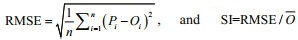
To verify the simulation ability of the SWAN model, we chose two of the most common and representative wind wave characteristics: the SWH and the mean wave period (MWP). The measured data were collected from three buoys, B1 (38.02°N, 119.51°E), B2 (39.30°N, 120.36°E) and B3 (38.09°N, 121.04°E), whose locations in the case are shown in Fig. 1. The comparisons between the simulations and observations of SWH and MWP are shown in Fig. 3. All of the SWH and the MWP time series basically follow a first increasing and then decreasing trend, with peak values occurring at similar times. The trends of the SWH and the MWP are well simulated by the established model. However, there are slight differences between both curves in magnitude. The SWAN simulations tend to underestimate the SWH at the peaks and underestimate the MWP where wave heights are relatively low at the initial stage of a cold wave.

|
| Figure 3 Simulated (blue lines) and observed (red crosses) time series of significant wave height and mean wave period induced by cold waves at the three buoys B1, B2 and B3 in December 2015 |
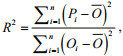
For a quantitative evaluation of the performance of the SWAN model, three error statistics, namely the mean error (ME), the root mean square error (RMSE), and the scatter index (SI), are adopted. The statistics are calculated as: 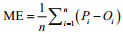
|
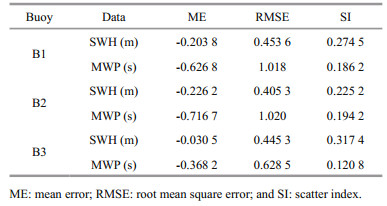
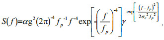
Since the SWAN model does not have any a priori restrictions on the spectrum for the evolution of wave growth, the spectral form should first be confirmed. A number of parametric forms of the wind wave frequency spectrum have been proposed to date. The best known and most widely used representation is the Joint North Sea Wave Project (JONSWAP) spectrum (Hasselmann et al., 1973):
 (1)
(1)The spectral shape parameter σc has little influence on the ultimate spectral form. Since previous fetchlimited studies have found no systematic trend within the scatter of values, this parameter has been assumed constant at σc=0.07 when f≤fp and σc =0.09 when f > fp. 
However, a significant amount of observation data in previous studies (e.g. Toba, 1973; Forristal, 1981; Kahma, 1981; Donelan et al., 1985) has suggested that an f-4 power law may be a better description of the rear face of the spectrum. Donelan et al. (1985) proposed a modified version of the JONSWAP spectrum:
 (2)
(2)For convenience, the form Eq.2 can be transformed into:
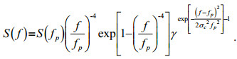 (3)
(3)fp and S(fp) can be easily obtained from the spectra. The value of γ was always set as the default average 3.3 or other empirical fixed values for practical application (Hasselmann et al., 1973; Ochi and Hubble, 1976; Young, 1998). This method is easy and efficient but brings deviations between the fitted spectra and the observations. In this study, the values of γ were obtained using the least-squares method to attain the best fits.
To analyze the results of the wave model simulations in detail, five different locations were selected, as illustrated in Fig. 1. Three points S1 (40.50°N, 121.50°E), S2 (39.00°N, 120.50°E) and S3 (37.50°N, 119.50°E) are distributed in the Bohai Sea. Two points S4 (39.50°N, 124.00°E) and S5 (38.00°N, 123.00°E) in the northern Yellow Sea. Based on Eq.3, some model and fitted spectra at each of the five sites are shown in Fig. 4. A uniform good fit to nearly all of the output spectra during the passage of the cold wave was attained with the modified JONSWAP spectral formulation by Donelan et al. (1985). It can be seen that, during the period of offshore wind in December 2015, the wave spectra are unimodal with similar shape and grow with time and space. As an obvious feature, although the wave spectrum S(f) is distributed between f=0 and f=∞ theoretically, a substantial part of the wave spectrum of cold wave-generated waves is concentrated in a narrow frequency band. In other words, the main part of the energy is provided by the wave components of the narrow band around the peak frequency. In fact, the studied area is smaller than the meteorological system of a cold wave, and the strong wind induced by the cold wave is relatively uniform and changes gently. Thus ocean waves induced by the cold wave are mainly wind waves, with the periods around 1/fp.

|
| Figure 4 Sample of the comparison between the six-hourly spectra (blue lines) and their equivalent modified JONSWAP spectral function (red lines) during the cold wave period in December 2015 at the five representative sites S1 to S5 |
The three characteristic parameters, fp, S(fp) and m0, can be used as the main indicators of spectral growth. Their time series at the five sites are shown in Fig. 5. For comparison, the wind speeds at 10 m above sea level, U10, at the five sites are also shown. S(fp) and m0 represent the maximum energy density and total wave energy of the wave spectrum, respectively. In the early stage of 10 December, when the strong and uniform cold-wave wind started to prevail in the NECS, S(fp) and m0 at the five sites all markedly increased. But on the contrary, regardless of the different initial values caused by previous sea states, peak frequencies fp all decreased slowly with time. Nonlinear interaction among composition waves of different frequencies is the main cause of this phenomenon. It continues delivering energy from medium to low frequencies, causing a peak to develop. It is worth mentioning that this is different from the sudden change in peak frequencies of hurricanegenerated wave spectra. As time went on, S(fp) and m0 both first increased and then decreased with the wind speed. They have the similar changing trends because of the typical narrow-band spectrum. At the peak time of S(fp) and m0, fp stopped to decrease and then remained essentially constant. fp at S1 and S4 is larger than that at S2, S3 and S5. This reveals that areas with a longer fetch tend to have a smaller peak frequency, and this finding is in agreement with the observed JONSWAP data (Hasselmann et al., 1973).

|
| Figure 5 Time series of 10-m wind speed U10, peak frequency fp, spectral peak S(fp) and spectral lowest moment m0 during the cold wave period at the five sites S1 to S5 Data for different sites are represented by different symbols. |
The growth of frequency spectra of cold-wave waves is considered by introducing parameters that directly or indirectly reflect the effect of wind field or other external environmental factors on the spectrum. In this section, dimensionless least-squares fits and log-log plots of the various wave spectral parameters against three universally used parameters, fetch (wind factor), inverse wave age (wave factor) and peak frequency (spectral factor) are presented and compared. The obtained growth relations of spectral parameters are valuable not only for the study of the growth mechanism of ocean waves, but also for the calculation and prediction of cold-wave waves.
4.1 Fetch dependencesAmong the various research methods, the wind wave growth relation is the most widely used and also an important basis of other related methods. International researchers have made considerable effort and proposed many fetch-limited growth relations to date (e.g. Mitsuyasu, 1968; Hasselmann et al., 1973; Davidan, 1980; Kahma, 1981; Donelan et al., 1985; Dobson et al., 1989; Wen et al., 1989; Ewans and Kibblewhite, 1990; Babanin and Soloviev, 1998) based on data from site investigations with different timescales in different seas. Most of the proposed relations reflect changes in the dimensionless peak frequency 


Using the above steps, the data for different sites are shown in Figs. 6, 7. The approximations of the dependences of 


 (4)
(4) (5)
(5)

|
Figure 6 Dependence of dimensionless peak frequency   |

|
Figure 7 Dependence of dimensionless wave energy   |
Equations 4 and 5, which are developed for fetchlimited waves, are remarkably good fits to the data and in good agreement with the experimental and observational dependences proposed in other studies. Besides, the wave height Hs and period Ts of significant waves can be calculated by the empirical relations: 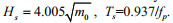

|
| Figure 8 Correlation between the dimensionless wave height H* and period T* of significant waves Different symbols represent the derived data from different sites; the black solid line is the 3/2 power law relationship presented by Toba (1972). |
Power-law regression has also been produced of dimensionless spectral peak 


|
Figure 9 Dependence of dimensionless spectral peak   |
 (6)
(6)The parameter S(fp), not like fp and m0, does not correspond to any external characteristic parameters of waves directly. That may be the reason why previous researchers rarely investigated it. Though the values of S(fp) can be easily known from data of spectra in the cases of hindcasting, the growth relation of S(fp) is of great importance for analyzing the growth of wave spectrum.
The peak enhancement factor γ represents the ratio of the spectral peak to the peak of the corresponding Pierson and Moskowitz spectrum at the same peak frequency. It not only characterizes the spectral peak properties, but also is an important measure of different wave development states. Hasselmann et al. (1973), in a careful study of fetch-limited waves, found no obvious relation between γ and 

 (7)
(7)

|
Figure 10 Dependences of the spectral peak enhancement factor γ on dimensionless fetch  |
It is the higher values of γ at large 

As the spectral forms developed from generation to generation, however, the constancy of α has been called into question. Special investigations have been carried out to study the behavior of the Phillips parameter α. Based on various observational and experimental data, the fetch-limited growth relation of α has been obtained (Hasselmann et al., 1973; Mitsuyasu et al., 1980; Dobson et al., 1989; Ewans and Kibblewhite, 1990; Babanin and Soloviev, 1998). However, since the experimental areas in previous studies are mostly open seas, the applicability of the previous derived relations in the NECS is weak. The parameter α is plotted against 
 (8)
(8)

|
Figure 11 Dependences of the Phillips parameter α on dimensionless fetch  |
It can be seen that the values of α at different sites are mainly in the range from 0.002 to 0.02, and show a regular decreasing trend with 
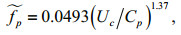
In practical applications, dimensionless fetch is more suitable for conditions when fetch is already known and the wind field remains relatively invariant. Cold wave cases are good examples for this, but there are many actual conditions when both wind speed and wind direction are always changing. Thus, some previous studies (e.g. Donelan et al., 1985; Dobson et al., 1989; Elfouhaily et al., 1997; Young, 1998) have used a more local wave parameter to describe the wave spectra: the inverse wave age Uc/Cp, where Uc represents U10 in the direction of the waves at the spectral peak and Cp represents the phase speed of those waves. As its name suggests, the inverse wave age is the reciprocal of wave age, which is well known to be an important wave factor reflecting wave growth states.
The time series of Uc/Cp at the five sites during the cold wave period are shown in Fig. 12. When the coldwave wind started to strengthen in the early hours of 10 December, waves in different areas all turned into a unified young state and values of Uc/Cp increased beyond 4.0. Subsequently, Uc/Cp gradually decreased to different extent. Elfouhaily et al. (1997) found that waves are fully developed, mature, developing and young when Uc/Cp≤0.83, 0.83 < Uc/Cp≤1.0, 1.0 < Uc/Cp≤2.0 and Uc/Cp>2.0, respectively. If we classify the waves during the cold wave using this standard, all data at S1, S3 and S4 and most data at S2 are young, while data at S5 are mostly developing and partly mature or developed. It is apparent that waves with a wider surface are more likely fully developed.

|
| Figure 12 Time series of inverse wave age Uc/Cp during the cold wave period at the five representative sites S1 to S5 Data for different sites are represented by different symbols. |
Donelan et al. (1985) analyzed the field data of the directional spectrum at steady state in an inland sea and related spectral parameters to Uc/Cp. For open-sea wave spectra in a variety of conditions, power-law regressions from Dobson et al. (1989) have also been produced. These previous obtained relations may be not suitable for wave spectra in this cold wave case. Hence, it is of great value to find the Uc/Cp dependences for this type of extreme weather in this study. Among the five sites, S3 should be treated differently. Since the special semi-enclosed terrain limits the development of waves, Uc/Cp is large at S3. However, the spectra at S3 have the long-fetch characteristics. Thence the growth relations of spectral parameters on Uc /Cp at S3 are significantly different from the other four sites. In Fig. 13, the data at site S3 are temporarily ignored to obtain dependences appropriate for the majority of the NECS. In Fig. 13a, b, c, the data still follow a power-law distribution and suggest the following relations:
 (9)
(9)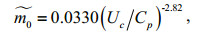 (10)
(10) (11)
(11)

|
Figure 13 Dependences of (a) dimensionless peak frequency    |
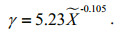
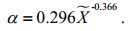
In Fig. 13d, e, there appears to be two trends for the different ranges of Uc/Cp. When the waves are young, γ and α show an increasing trend respectively with Uc /Cp; when the waves start to develop, γ and α seem to be fairly constant or show a slowly varying trend. Thus, relations linking the two shape parameters to Uc /Cp are obtained with least-squares fitted piecewise functions:
 (12)
(12) (13)
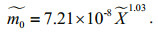
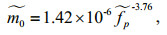
(13)The peak frequency fp is the most characteristic, accurately defined and easily measured variable of the wave spectrum. It varies slowly during the spectrum development and can reflect the wave development stage. Mitsuyasu et al. (1980) first tried to use fp to determine other spectral parameters m0, γ and α, but the observed data were very sparse. Babanin and Soloviev (1998) also examined the interrelationships of the spectral parameters with in situ data in the Black Sea. Since the dependence of 


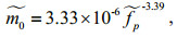 (14)
(14)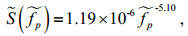 (15)
(15)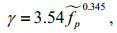 (16)
(16)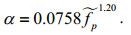 (17)
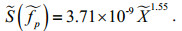
(17)These relations Eqs.14–17 are compared in Fig. 14 with the dimensionless spectral data and the fitted dependences:
 (18)
(18) (19)
(19) (20)
(20) (21)
(21)

|
Figure 14 Dependences of (a) dimensionless wave energy    |
The data have strong dependences on 
From the above arguments, three groups of empirical relations describing the growth of wave spectral parameters (


|
On the whole, it can be validated that the power equation is good for fitting the relationships between the spectral parameters and development factors. The good agreement of our results with those of other investigators suggests the universal character of the dependence describing variability of the parameters of fp, S(fp) and m0. Dependences on the inverse wave age during the extreme weather system like cold wave are different from the ordinary-wind condition and need a special treat.
5 SUMMARY AND CONCLUSIONAs studies of wind waves, frequency spectra and growth relations have been undertaken before, we point out that this article is a systematic study of typical conditions in the semi-enclosed NECS during a cold wave. In the NECS, cold waves are more frequent and more harmful than typhoons or other extreme weather events, and the effect of cold waves on the ocean environment, such as strong winds and giant waves, is one of the most important marine natural disasters. Thus, the study of wind wave spectra is imperative for forecasting the rough seas generated by cold waves, and provides a scientific foundation for disaster prevention and mitigation, marine hydrological security, and resource development and utilization.
A typical wave action model, SWAN, was used to simulate ocean waves and output frequency spectra. A representative cold-wave case was investigated. The spatiotemporal characteristics of the wind field and wave field show that cold wave seas in the NECS are mostly local wind-generated waves and are influenced by both winds and terrains. Despite errors from the wind forcing data, good agreement is found between model results and measurements not only in magnitudes but also in phases, thus the output data are reliable for spectral studies. Based on data from five selected sites, the wave spectra during the passage of a cold wave show only one significant peak and appear to be well-fitted by the modified JONSWAP parametric spectral form proposed by Donelan et al. (1985). The spectra grow with time and space, and are reflected by peak frequency, spectral peak and lowest moment. The three characteristic parameters change with the wind field in the temporal dimension and vary with fetch in the spatial dimension.
The growth relations of spectral parameters are established to study the development of the cold wave-generated spectra. In all of our analyses, we used log-log plots to relate the physically dependent variables (dimensionless peak frequency 


The datasets used during the model configuration are available in the ETOPO-5 repository (http://www.ngdc.noaa.gov/mgg/fliers/93mgg01.html) and CFSR repository (http://cfs.ncep.noaa.gov/cfsr/). The spectral data generated during the current study are available from the corresponding author on reasonable request.
7 ACKNOWLEDGEMENTWe thank North China Sea Marine Forecasting center of State Oceanic Administration for providing the measured data collected from the buoys and assisting in model verification.
Babanin A V, Soloviev Y P. 1998. Field investigation of transformation of the wind wave frequency spectrum with fetch and the stage of development. J. Phys. Oceanogr., 28(4): 563-576.
DOI:10.1175/1520-0485(1998)028<0563:FIOTOT>2.0.CO;2 |
Booij N, Ris R C, Holthuijsen L H. 1999. A third-generation wave model for coastal regions:Ⅰ.Model description and validation. J. Geophys. Res., 104(C4): 7649-7666.
DOI:10.1029/98JC02622 |
Davidan I N. 1980. Investigation of wave probability structure on field data. Trudi GOIN, 151: 8-26.
|
Deng Z A, Xie L A, Han G J, Zhang X F, Wu K J. 2012. The effect of Coriolis-Stokes forcing on upper ocean circulation in a two-way coupled wave-current model. Chin. J. Oceanol. Limnol., 30(2): 321-335.
DOI:10.1007/s00343-012-1069-z |
Ding Y H, Krishnamurti T N. 1987. Heat budget of the Siberian high and the winter monsoon. Mon. Wea. Rev., 115(10): 2428-2449.
DOI:10.1175/1520-0493(1987)115<2428:HBOTSH>2.0.CO;2 |
Dobson F, Perrie W, Toulany B. 1989. On the deep-water fetch laws for wind-generated surface gravity waves. Atmos.-Ocean, 27(1): 210-236.
DOI:10.1080/07055900.1989.9649334 |
Donelan M A, Hamilton J, Hui W H. 1985. Directional spectra of wind-generated waves. Philos. Trans. Roy. Soc. A, 315(1534): 509-562.
DOI:10.1098/rsta.1985.0054 |
Elfouhaily T, Chapron B, Katsaros K, Vandemark D. 1997. A unified directional spectrum for long and short winddriven waves. J. Geophys. Res., 102(C7): 15781-15796.
DOI:10.1029/97JC00467 |
Ewans K C, Kibblewhite A C. 1990. An examination of fetchlimited wave growth off the west coast of New Zealand by a comparison with the JONSWAP results. J. Phys. Oceanogr., 20(9): 1278-1296.
DOI:10.1175/1520-0485(1990)020<1278:AEOFLW>2.0.CO;2 |
Forristall G Z. 1981. Measurements of a saturated range in ocean wave spectra. J. Geophys. Res., 86(C9): 8075-8084.
DOI:10.1029/JC086iC09p08075 |
Gorman R M, Neilson C G. 1999. Modelling shallow water wave generation and transformation in an intertidal estuary. Coast. Eng., 36(3): 197-217.
DOI:10.1016/S0378-3839(99)00006-X |
Guan C L, Sun Q. 2002. Analytically derived wind wave growth relations. China Ocean Eng., 16(3): 359-368.
|
Hasselmann K, Barnett T P, Bouws E, Carlson H, Cartwright D E, Enke K, Ewing J A, Gienapp H, Hasselmann D E, Kruseman P, Meerburg A, Muller P, Olbers D J, Richter K, Sell W, Walden H. 1973. Measurements of wind-wave growth and swell decay during the Joint North Sea Wave Project (JONSWAP). Deutches Hydrographisches Institut, Hamburg. 95p.
|
Huang B G. 2008. Numerical simulation of waves in Bohai Sea and research on the influence of swells on wind waves. M.S. thesis, Ocean Univ. of China, Qingdao, Shandong, China. p.1-59. (in Chinese)
|
Jin K R, Ji Z G. 2001. Calibration and verification of a spectral wind-wave model for Lake Okeechobee. Ocean Eng., 28(5): 571-584.
DOI:10.1016/S0029-8018(00)00009-3 |
Kahma K K. 1981. A study of the growth of the wave spectrum with fetch. J. Phys. Oceanogr., 11(11): 1503-1515.
DOI:10.1175/1520-0485(1981)011<1503:ASOTGO>2.0.CO;2 |
Komen G J, Hasselmann S, Hasselmann K. 1984. On the existence of a fully developed wind-sea spectrum. J. Phys. Oceanogr., 14(8): 1271-1285.
DOI:10.1175/1520-0485(1984)014<1271:OTEOAF>2.0.CO;2 |
Liu T J, Zheng C W, Zhou L, Wu H X, Zhang H. 2013. Analysis on a cold air wave by using QN mixed wind data and SWAN model. Meteorological, Hydrological and Marine Instruments, 30(3): 8-12.
(in Chinese with English abstract) |
Mitsuyasu H, Tasai F, Suhara T, Mizuno S, Ohkusu M, Honda T, Rikiishi K. 1980. Observation of the power spectrum of ocean waves using a cloverleaf buoy. J. Phys. Oceanogr., 10(2): 286-296.
DOI:10.1175/1520-0485(1980)010<0286:OOTPSO>2.0.CO;2 |
Mitsuyasu H. 1968. On the growth of the spectrum of windgenerated waves (Ⅰ). Rep. Res. Inst. Appl. Mech., Kyushu Univ., 16: 459-482.
|
Mo D X, Hou Y J, Li J, Liu Y H. 2016. Study on the storm surges induced by cold waves in the Northern East China Sea. J. Mar. Syst., 160: 26-39.
DOI:10.1016/j.jmarsys.2016.04.002 |
Ochi M K, Hubble E N. 1976. On six-parameter wave spectra. In: Proceedings of 15th International Conference on Coastal Engineering, 1: 301-328.
|
Pan Z D, Sun L T, Hua F, Yuan Y L. 1992. LAGFD-Ⅱ regional numerical wave model and its application Ⅱ. Characteristics inlaid computational scheme. Oceanologia et Limnologia Sinica, 23(5): 460-467.
(in Chinese with English abstract) |
Ris R C, Holthuijsen L H, Booij N. 1999. A third-generation wave model for coastal regions:2. Verification. J. Geophys. Res., 104(C4): 7667-7681.
DOI:10.1029/1998JC900123 |
Rogers W E, Hwang P A, Wang D W. 2003. Investigation of wave growth and decay in the SWAN model:three regional-scale applications. J. Phys. Oceanogr., 33(2): 366-389.
DOI:10.1175/1520-0485(2003)033<0366:IOWGAD>2.0.CO;2 |
Toba Y. 1972. Local balance in the air-sea boundary processes Ⅰ. On the growth process of wind waves. J. Oceanogr., 28(3): 109-120.
DOI:10.1007/BF02109772 |
Toba Y. 1973. Local balance in the air-sea boundary processes Ⅲ. On the spectrum of wind waves. J. Oceanogr. Soc. Japan, 29(5): 209-220.
DOI:10.1007/BF02108528 |
Wen S C, Zhang D C, Guo P F, Chen B H. 1989. Parameters in wind-wave frequency spectra and their bearings on spectrum forms and growth. Acta Oceanologica Sinica, 8(1): 15-39.
|
Wu J. 1982. Wind-stress coefficients over sea surface from breeze to hurricane. J. Geophys. Res., 87(C12): 9704-9706.
DOI:10.1029/JC087iC12p09704 |
Yang D Z. 2004. Investigation of numerical forecasting wave model in Bohai Sea. M.S. thesis, Institute of Oceanology, Chinese Academy of Sciences, Qingdao, Shandong, China. p.1-59. (in Chinese)
|
Yao Q, Zheng C W, Su Q, Wang J, Liang X Y, Li Y B. 2013. Simulation of wave field in the China Sea by using WAVEWATCH Ⅲ wave model. Marine Forecasts, 30(2): 49-54.
(in Chinese with English abstract) |
Young I R. 1998. Observations of the spectra of hurricane generated waves. Ocean Eng., 25(4-5): 261-276.
DOI:10.1016/S0029-8018(97)00011-5 |
Zheng G D, Zhao H J, Xu F M, Zhang S H. 2010. Numerical simulation of wind waves in Bohai Sea induced by "98.04" cold wave. Port & Waterway Engineering, (2): 36-39.
(in Chinese with English abstract) |