 2019, Vol. 37
Institute of Oceanology, Chinese Academy of Sciences
Article Information
- JIANG Xingjie, GUAN Changlong, WANG Daolong
- Rogue waves during Typhoon Trami in the East China Sea
- Journal of Oceanology and Limnology, 37(6): 1817-1836
- http://dx.doi.org/10.1007/s00343-019-8256-0
Article History
- Received Sep. 25, 2018
- accepted in principle Nov. 28, 2018
- accepted for publication Mar. 19, 2019


2 Ocean University of China, Qingdao 266071, China
Rogue waves are wind-generated sea waves that are considerably higher than the surrounding waves. A traditional definition of a rogue wave is Hmax/Hs > 2 (Dysthe et al., 2008; Kharif et al., 2009), where Hmax is the maximum wave height in a certain wave field and Hs is the significant wave height. Various theories have been proposed to explain the formation of rogue waves (Kharif and Pelinovsky, 2003; Kharif et al., 2009) including ⅰ) nonlinear focusing due to third-order quasi-resonant wave-wave interaction (Janssen, 2003) and ⅱ) purely dispersive focusing due to second-order nonresonant or bound harmonic waves, which does not satisfy the linear dispersion relation (Fedele, 2008; Fedele and Tayfun, 2009). Both theories include complex nonlinear effects but their physical mechanisms operate in different sea state conditions.
Third-order quasi-resonant interactions and associated modulational instabilities are observed more easily in a sea state where wave energy is concentrated in direction and frequency (Janssen and Bidlot, 2009; Mori et al., 2011; Fedele, 2015) and the water depth influences the modulational instabilities (Janssen and Onorato, 2007; Janssen and Bidlot, 2009; Janssen, 2018), too. Some rogue waves do indeed occur in sea states with concentrated energy distributions (Waseda et al., 2012, 2014) but some occur under completely different conditions (Fedele et al., 2016, 2017). Purely dispersive focusing is more likely to occur in a sea state dominated by second-order nonlinearities (Tayfun and Fedele, 2007; Fedele, 2008). However, the questions of whether second-order nonlinearities dominate the dynamical process of rogue waves or whether third-order nonlinearities also play an important role remain under discussion (Fedele et al., 2016, 2017).
It is evident that the sea state condition is important in the formation of rogue waves. With current wave modeling technology, large-scale sea state simulation still depends on third-generation wave models. Largescale spatiotemporal simulation can elucidate wave field evolution including the evolution of wave systems; however, the directional spectra simulated by such models tend to smooth the information on both wave phase and surface elevation, which are crucial for rogue waves. Although directional spectra remain the basis of rogue wave research, it is inadequate to simply consider only bulk parameters like significant wave height and mean wave period integrated from the spectra.
This study investigated the sea state conditions pertaining at the time three rogue waves were observed during Typhoon Trami in the East China Sea in 2013. The third-generation WAVEWATCH Ⅲ model (The WAVEWATCH Ⅲ Development Group (WW3DG), 2016) was adopted to simulate the sea state conditions and spectra. The evolution of wave systems in the region of the observations was analyzed using an algorithm for spatial and temporal wave system tracking (Hanson and Phillips, 2001; Devaliere et al., 2009). Furthermore, taking advantage of the High-Order Spectral (HOS) method (Ducrozet et al., 2016), wave surface elevations were simulated and used to determine the relative importance of nonlinearities. Certain characteristic parameters of the two theories mentioned above were selected to assess whether such physical mechanisms were in operation during the studied events.
The remainder of this paper is organized as follows. In Section 2, the records of the observed rogue waves and the meteorological conditions pertaining at the time of their occurrence are introduced, and the methodology used in the analysis is described. The simulated results and analyses are presented in Section 3. Finally, our conclusions are offered in Section 4.
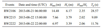
2 MATERIAL AND METHOD 2.1 Observational records and meteorological conditionsIn August 2013, three rogue wave events Hmax/Hs > 2 were recorded by a wave buoy located at 29.068 7°N, 124.921 5°E, with a local water depth of about 88 m. The TRIAXYSTM Directional Wave Buoy (AXYS Technologies Inc., Canada) recorded horizontal and vertical displacement of the water surface hourly with a sampling interval of 0.78 s (i.e., 1.28 Hz). Details of the recorded rogue waves are shown in Table 1.
The time series of normalized profiles of the three rogue waves are shown in Fig. 1. Much sharper crests are evident accompanied by asymmetric troughs at the time of the occurrence of the maximum elevations (locating at 0 of the x-axes of Fig. 1), denoting significant nonlinear effects. Moreover, the influence of external forces such as fishing-boat dragging or a signal fault of the instrument can be excluded based on Fig. 1.

|
| Fig.1 Time series of normalized profiles of recorded rogue waves |
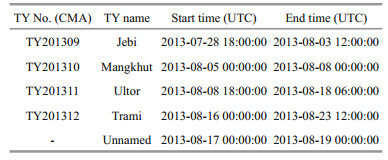
According to the tropical cyclone database of the China Meteorological Administration (tcdata. typhoon.org.cn) (Ying et al., 2014), all three rogue waves might have been affected primarily by Typhoon Trami (Table 2 and Fig. 2). When event RW2106 occurred, Trami was generating large waves near the observation site, but when the final two events (i.e., RW2215 and RW2222) occurred, Trami's center had made landfall to the southwest of the observation site. Several other typhoons mentioned in Table 2 had become tropical depressions before the studied events occurred. In August, the prevailing wind in the South China Sea is from the southwest, while that in the East China Sea is from the south and southwest.
|

|
| Fig.2 Nested grid settings of WAVEWATCH Ⅲ and tracks of typhoons that might have influenced the studied rogue wave events |
The third-generation WAVEWATCH Ⅲ model (Tolman, 1991) version 5.16 (The WAVEWATCH Ⅲ Development Group (WW3DG), 2016) was used to simulate the wave field and to track the wave systems (Section 2.2.2). The spectra used as initial conditions of the HOS method simulation (Section 2.2.3) and in the assessment of certain characteristic parameters (Section 2.2.4) were also derived from the wave model. Thus, all of the results based on the same numerical modeling were consistent.
The spectral space of WAVEWATCH Ⅲ was set as 36 directions with intervals of 10 degrees and 35 frequencies logarithmically spaced from the minimum frequency 0.042 Hz up to 1.05 Hz with intervals of fi+1/fi=1.1. In the current version of WAVEWATCH Ⅲ, several input (Sin) and dissipation (Sds) source term packages have been provided to model the wave fields. In this study, the ST4 source package (Ardhuin et al., 2010) was adopted, which had performed better than other Sin+Sds combinations in our previous experiments with current settings of the model. And the nonlinear wave-wave interactions were parameterized by the DIA method (Hasselman et al., 1985) in the model.
With consideration of the swells generated by non-local wind systems and because the prevailing winds were from south and southwest, the southern border of our computational grid extended to 5°N and the western border extended to 100°E. The parent computational grid (5°–45°N, 100°–150°E) also covered the tracks of the typhoons listed in Table 2. In anticipation of high resolution for the wave system tracking, we designed a set of three nested grids (see Fig. 2): nst0, ns1, and nst2 with resolutions of 1/4°, 1/8°, and 1/16°, respectively. The bathymetric data were obtained from the ETOPO1 1 Arc-Minute Global Relief Model (DOI: 10.7289/V5c8276m) of the National Centers for Environmental Information of the National Oceanic and Atmospheric Administration, and the depth read from the ETOPO1 at the observation site was 89 m, which was considered sufficiently precise for the numerical simulation. Finally, no wave level change was considered because the effect of wave level changing was negligible for the local water depth.
The CFSv2 Selected Hourly Time-Series Products (Saha et al., 2011) were used to drive the wave model. With consideration of the typhoon tracks and the non-local wind systems, we decided to allow sufficient time for waves to develop before the occurrence of the first rogue wave and to see how the sea state might be changed after the occurrence of the final event. Thus, the numerical simulation was executed from 20130810 00:00:00 to 20130824 00:00:00 (all dates and times used in this paper are referred to UTC).
2.2.2 Spatial and temporal tracking of wave systemsA wave field might comprise one wind sea system generated by local winds and several swell systems generated by distant storms. The composition of a wave system could play an important role in the formation of a rogue wave. Since version 4.08, wave system tracking postprocessing has been available in the WAVEWATCH Ⅲ source code package. Based on the spectral partitioning procedure (Vincent and Soille, 1991; Hanson and Jensen, 2004; Hanson et al., 2009), some spatial and temporal correlation steps have been introduced (Voorrips et al., 1997; Hanson and Phillips 2001; Devaliere et al., 2009) to track the spatial and temporal changes of a certain spectral partition (wave system). Taking advantage of this tracking can provide visualization of the process of generation, coexistence, and diminishment of wave systems for a single point or within a certain area. Although the accuracy might be influenced by the computational resolution or by the parameters of the algorithm, the trend of variation of the wave systems can still be elucidated.
2.2.3 High-Order Spectral methodNonlinear effects are important in the formation of rogue waves. The two most popular theories on how rogue waves occur have a very close relationship with the order of nonlinearity. Modulational instability is induced by third-order quasi-resonant wave-wave interactions (Janssen, 2003), while purely dispersive focusing is caused by second-order nonresonant or bound harmonic waves (Fedele, 2008; Fedele and Tayfun, 2009). Thus, the order of nonlinearity that dominates the wave field might indicate the possible physical mechanism behind the occurrence of a rogue wave.
High-order statistical characteristics of wave surface elevations such as skewness and kurtosis denote the nonlinear effects of a given wave field. However, it is widely known that the directional spectra of such wave fields simulated by third-generation wave models have smoothed signals of wave phase and surface elevation. To represent those signals again, highly and fully nonlinear potential flow solvers must be applied. The HOS method pseudo-spectral numerical algorithm (Dommermuth and Yue, 1987; West et al., 1987) represents a potential flow solver with acceptable efficiency and accuracy. Based on a perturbation expansion of the wave potential function up to a prescribed M order of nonlinearities in terms of a small parameter, the HOS method can be used to solve for nonlinear wave-wave interactions up to the specified order M.
As the potential flow solver, this study adopted the HOS-ocean software version 1.5 (Ducrozet et al., 2016). The suitability of HOS-ocean has been verified in studies of modulational instability (Toffoli et al., 2010; Fernandez et al., 2014) and rogue waves (Ducrozet et al., 2007; Sergeeva and Slunyaev, 2013; Xiao et al., 2013). Potential flow solvers are limited to nonbreaking waves, but if the wave field presents marginal breaking that is highly localized in space and time, the simulation might be able to continue. Considering this limitation (Ducrozet et al., 2017), the wave field was resolved with the spatial discretization of Nx×Ny=192×192 points (total number of points: 384×384) on a 2 km×2 km area and temporal duration of 1 800 s. With consideration of that, the simulated peak wavelengths of the sea states where three events occurred are 240, 200, 160 m respectively, such settings allowed accurate estimation of the possible presence of wave breaking and the energy dissipation due to wave breaking could be neglected. In consideration of the spatial-temporal scales in this study, the growth of waves due to wind input is practically insignificant (Dysthe et al., 2003; Janssen, 2003), thus the wind effect was ignored too. Furthermore, only constant water depth was considered in the simulations.
Initial conditions for the wave potential and surface elevation were specified from the directional spectra output by the WAVEWATCH Ⅲ simulation at the moments and locations when and where the rogue waves occurred. The HOS-ocean nonlinear order was set separately as M=3 and M=2. If no discrepancies were observed, second-order nonlinearities were dominant; otherwise, third-order nonlinearities had a reasonably important role. For each order M, the HOS-ocean simulation was performed 50 times, and the mean value and 95% confidence interval were considered to ensure coherence of the HOS-ocean simulation runs.
2.2.4 Characteristic parameters of sea stateCertain characteristic parameters based on the geometry of a directional spectrum denote the status of a sea state condition that is closely related to the formation and occurrence probability of rogue waves. Based on the spectra output by WAVEWATCH Ⅲ, this study estimated four sets of such parameters. Single values of these parameters might be meaningless in relation to the entire physical process; however, their relative differences and trends of variation at each stage of the process illustrate further details of the rogue waves. Discussion on the physical significance of those parameters and on how best they could be estimated is presented in Section 3.4.
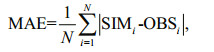
3 RESULT 3.1 Numerical simulation of the wave fieldIllustrations of the acceptable performance of the simulation of bulk parameters, e.g., significant wave height, mean cross-zero wave period and mean wave direction, are shown in Fig. 3a with vertical dashed lines identifying the times at which the rogue waves occurred. And the mean absolute errors (MAE) between observed and simulated parameters are listed in Table 3 and calculated as
 (1)
(1)

|
| Fig.3a Comparison of simulated results and observations Vertical dashed lines indicate the hours at which the rogue waves occurred. |

where N is the number of total samples, OBSi and SIMi are the ith observed and simulated parameters in their respective time series which are synchronous. The corresponding CSFv2 wind speed and direction at the observation site are shown in Fig. 3b.

|
| Fig.3b Wind speed and direction of the CFSv2 products at the observation site |
The wave and wind fields at the times of occurrence of the rogue waves are shown in Fig. 4a–f. At 06:00 on 21 August 2013, Typhoon Trami was centered near the northeastern corner of the Taiwan, China, with its area of maximum wind speed of > 20 m/s located at approximately 27.5°N, 122.5°E (Fig. 4d). Similarly, the maximum significant wave height of > 7 m can also be seen at the same location, which was very close to the observation site (Fig. 4a). The maximum simulated significant wave height at the observation site was 6.13 m, the mean direction of the waves was toward NW and the corresponding wind direction was toward WNW. Thus, it can be inferred that event RW2106 occurred in a wave field that was influenced intensely by the typhoon.

|
| Fig.4 Simulated (a–c) wave and (d–f) wind fields at the times when the rogue waves occurred Observation site is marked as "+". |
The wind and wave fields at the times when events RW2215 and RW2222 occurred are shown in Fig. 4b and e and Fig. 4c and f, respectively. Typhoon Trami had made landfall before event RW2215 occurred. At this time, the wind direction at the observation site was toward NNW, mean wave direction was toward N and simulated significant wave heights were 3.77 and 3.50 m. The area of maximum significant wave height, which had reduced to approximately 3–4 m, was located at 28°–29°N, 122.5°E at the end of the wind fetch and not far from the observation site. In comparison with event RW2106, the influence of Trami in the region of the observation site had weakened considerably during the final two events.
The PM spectrum (Pierson and Moskowitz, 1964) which presents fully developed sea states was adopted to assess the degree of development of the sea states where the rogue waves occurred. The peak period of the PM spectrum is
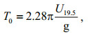 (2)
(2)where U19.5 is the wind speed at 19.5 m above the sea surface and g is the gravitational acceleration (=9.81 m/s2). Because the u-v wind data used in the CFSv2 dataset is at 10 m, a simple transformation needed to be applied
 (3)
(3)The T0s of the three events and related parameters are shown in Table 4. It can be seen that the simulated peak period (Tp) of events RW2215 and RW2222 are much larger than PM peaks under the wind speed at the time when the two events occurred, denoting those two events occurred in fully developed sea states. However, Tp of event RW2106 is a little smaller than the T0 assessed under the corresponding wind speed, implying that the sea state might have not completely developed at that time. With consideration of that the simulated Hs and Tp were attaining the peak of the whole process at the time of the occurrence of event RW2106 (see Fig. 3a) and the conclusion we have drawn that the sea state was intensely influenced by the typhoon at that time, it is inferred that the sea state was quasi-fully developed where event RW2106 occurred.

|
The wave system tracking in WAVEWATCH Ⅲ was used to track the evolution of the wave systems at the observation site and in the area covered by nst2 (20.0°–33.0°N, 120.0°–130.0°E). Detected wave systems are shown in the upper subplot with different colors and the wind-sea and swell systems in coexistence can be easily identified by their peak periods which are usually larger for swell systems. The magnitude of each vector represents the significant wave height of each system and the direction of that represents which direction the system is propagating to. Similar representation for local wind is illustrated in the lower part of Fig. 5.

|
| Fig.5 Wave systems and wind vectors at the observation site |
As shown in Fig. 5, system sys-1 (black arrows) was present for all three events. Based on the wind vector shown in the lower part of Fig. 5 and the previous analysis of the wind and wave fields, sys-1 represents the dominant wind sea system of Typhoon Trami. The system sys-2 (blue arrows), which was in existence before sys-1, i.e., during August 16–18, might represent the influence of the "unnamed" tropical depression (see Fig. 2 and Table 2).
Only one wind sea system was evident at the observation point when event RW2215 occurred, although the mean wave direction deviated slightly from the local wind direction (Fig. 5). At the time of event RW2222, two systems were in coexistence: one toward NW (in the same direction as the wind) and the other toward NE. After the occurrence of the final event, wave systems in the region of the observation site became much more complex, and the wind sea system no longer reflected a single wave system.
The outputs of the tracking algorithm could help elucidate the evolution of the wave systems; however, inaccuracies can occur when the significant wave height or peak period of different systems are similar. This situation was in existence when events RW2215 and RW2222 occurred because the wind and wave fields were both in a transitional period as the influence of Typhoon Trami diminished. As shown in Fig. 6, two systems were present in the region of the observation site when event RW2215 occurred, both with a significant wave height of 4–5 m in peak period of 10–12 s. The primary difference between the two systems was the wave direction (sys-1 and sys-3). The system with wave direction toward NW and the system with wave direction toward NE both influenced the observation site at the moment event RW2215 occurred. A similar situation can be observed in Fig. 7 at the time when event RW2222 occurred (sys-1 and sys-4).

|
| Fig.6 Wave systems in the region of the observation site at 15:00:00 on 20180822 |

|
| Fig.7 Wave systems in the region of the observation site at 22:00:00 on 20180822 |
Based on the above analysis, we conclude that Typhoon Trami affected all three events but to differing degrees. For event RW2106, the storm was powerful and the wave field was dominated totally by its wind sea system. As Trami made landfall, the storm diminished to a tropical depression and weakening of its influence was inevitable. Events RW2215 and RW2222 occurred near the end of the storm when another system with a wave direction different from the local wind developed and gradually became increasingly stable. According to the wave direction, this new system was probably generated by the southwest wind in the southern East China Sea. Furthermore, the spectrum of event RW2106 might have had a narrower directional distribution than events RW2215 and RW2222, which implies a greater probability of triggering modulational instability.
3.3 HOS simulationHigh-order statistics of water surface elevation η such as skewness λ3 and excess kurtosis λ40 denote the importance of the nonlinearity of sea state:
 (4)
(4)where < > means the statistical average and σ is the standard deviation of surface wave elevation. Skewness is contributed totally by second-order bound waves (Tayfun, 1980; Tayfun and Fedele, 2007; Fedele and Tayfun, 2009), whereas excess kurtosis includes a dynamical part λ40d, which represents contributions from third-order nonlinear quasi-resonant wave-wave interactions (Janssen, 2003; Janssen and Bidlot, 2009) and a bound part λ40b that represents contributions from crest-trough asymmetry caused by both second- and third-order nonlinearities (Tayfun, 1980; Tayfun and Lo, 1990; Tayfun and Fedele, 2007; Fedele, 2008; Fedele and Tayfun, 2009; Janssen, 2009; Janssen and Bidlot, 2009):
 (5)
(5)Numerical simulations of HOS-ocean were performed with settings of M=2 (considering only second-order nonlinearities) and M=3 (both second- and third-order nonlinearities) using the WAVEWATCH Ⅲ simulated directional spectrum as initial conditions. The time evolutions of statistical skewness and excess kurtosis of the 50 runs for each value of M (M=2: black, M=3: red) and for each event are shown in Fig. 8 (RW2106: Fig. 8a & d, RW2215: Fig. 8b & e, and RW2222: Fig. 8c & f). Solid lines in Fig. 8 are the mean values and dashed lines are the 95% confidence bands; blue lines are theoretical values of skewness and kurtosis in a narrow band condition, which is discussed in Section 3.4.

|
| Fig.8 Time evolution of skewness λ3 and excess kurtosis λ40 based on HOS-ocean simulated surface elevation for event RW2106 (a and d), RW2215 (b and e) and RW2222 (c and f) |
An artificial transient period of about 100 s can be seen in each subplot of Fig. 8, which is introduced for the relaxation scheme (Dommermuth, 2000) to stabilize the transition from linear initial conditions to a fully nonlinear calculation. The value of λ3 should be contributed totally by second-order bound waves; therefore, no discrepancies between the black and red lines are evident in Fig. 8a–c, i.e., the third-order nonlinearity had nothing to do with skewness. As mentioned at the end of Section 3.2, event RW2106 might have had a greater likelihood of being affected by the modulational instability. However, there is no obvious departure of λ40 based on M=2 and 3 in Fig. 8d, and similar situations can be seen in Fig. 8e & f. Thus, third-order quasi-resonant wave-wave interactions did not play an important role in the formation of any of the three rogue wave events, and the pertaining sea states were all dominated by second-order nonlinearities. As for the relative values of λ3 and λ40, the statistical parameters of event RW2106 are slightly larger than events RW2215 and RW2222, which means more significant deviation from the Gaussian structure of linear seas and an increased occurrence of large waves.
3.4 Characteristic parametersIn this section, characteristic parameters based on the geometry of the directional spectra simulated using the WAVEWATCH Ⅲ model are presented. Further details of the sea states and nonlinear effects are discussed and the reason why the modulational instability was not the primary factor in the formation of the observed rogue waves is illustrated. The characteristic parameters are introduced as:
3.4.1 Freakish sea indexThe freakish sea index maps the trajectory of the directional spreading σθ (Kuik et al., 1988) and frequency bandwidth Qp (Goda, 1970), and it has been used successfully in studies of the Suwa-Maru incident (Tamura et al., 2009) and the Onomichi-Maru incident (In et al., 2009):
 (6)
(6) (7)
(7)where S(ω, θ) is the directional spectrum with 
The mean wavelength Lx and mean wave crest length Ly can be expressed as follows (Baxevani and Rychlik, 2006; Fedele, 2012):
 (8)
(8)where mijl is the moment of a spectrum S(ω, θ) and mijl=∫kxikyjωlS(ω, θ)dωdθ where the x direction is the direction of wave propagation and the y direction is vertical to the x direction. The degree of short crestedness can be expressed as:
 (9)
(9)which in sea states with long crestedness tends toward 0 and in sea states with short crestedness tends toward 1 (Longuet-Higgins, 1957). The irregularity parameters (Baxevani and Rychlik, 2006; Fedele, 2012):
 (10)
(10)express the correlation between gradients of sea surface elevation along spatial and temporal coordinates. The irregularity parameters account for the correlation between space and time (αxt and αyt) or space and space (αxy) of sea surface gradients. They can assume absolute values within the range 0–1 that correspond to "confused" and "organized" sea state conditions, respectively (Barbariol et al., 2015).
3.4.3 Theoretical skewness and kurtosis in a narrowband conditionWhen discussing the consequences of the canonical transformation in the Hamiltonian theory of water waves (Zakharov, 1968) using Krasitskii's canonical transformation, general expressions for the skewness and the kurtosis of the sea surface have been proposed (Janssen, 2009; 2018). The general expressions are complex but they can be simplified in narrowband conditions (Tayfun, 2006; Janssen, 2009) and fitted for moderate finite depth:
 (11)
(11)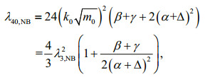 (12)
(12)with
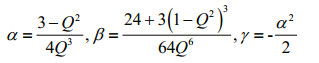
and
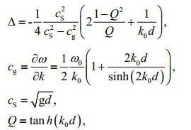 (13)
(13)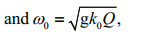 (14)
(14)where d is the local depth, k0 is the theoretically dominant wave number and 
To improve the performance of the ECMWF freak wave warning system (ECMWF, 2016), new parametrizations of skewness and kurtosis of the envelope wave height (Janssen, 2014; Janssen and Bidlot, 2009) have been presented (Janssen, 2018). Envelope skewness and kurtosis are important factors used to depict the maximum envelope wave height distribution for weakly nonlinear systems, and these two parameters and other associated variables can reveal further details of sea state (Janssen, 2009, 2018; Janssen and Bidlot, 2009) though they are not the real skewness and kurtosis of a certain sea state. The parametrizations were validated by numerical experiments on the Draupner wave and the Andrea Storm. In this paper, we use exactly the same expressions and free parameter choices as in ECMWF Technical Memorandum 813 (Janssen, 2018) except the dynamical kurtosis expression which followed Fedele's work (Fedele, 2015).
The envelope wave height theory (Janssen, 2009; Janssen and Bidlot, 2009; Janssen, 2014, 2018) also includes a skewness parameter C3 that represents the contributions solely from second-order bound waves and a kurtosis parameter C4, which has a dynamical part C4dyn and a bound part C4bound, which represent the contributions of third-order quasi-resonant wavewave interactions and the contributions of both second- and third-order bound waves, respectively:
 (15)
(15) (16)
(16)The definitions of α, γ and Δ in Eqs.15–16 are similar to Eq.13 but with an extra term that expresses the effect of shallow water. The term 
The dynamical part of envelope kurtosis C4dyn is associated with the modulational instability due to third-order quasi-resonant wave-wave nonlinear interactions (Janssen, 2003; Mori and Janssen, 2006; Janssen and Onorato, 2007; Janssen and Bidlot, 2009; Mori et al., 2011; Fedele, 2015) and influenced by the relative directional width and local water depth. With a Gaussian type directional spectrum, Fedele (2015) derived the dynamical kurtosis analytically under the narrowband assumption. The results show that, in the focusing regime (0 < R < 1, where R is an important parameter discussed later), the C4dyn of an initially homogeneous Gaussian wave field grows, attaining a maximum at an intrinsic time scale. Thus, the sea state initially deviates from being Gaussian, but eventually, the dynamical kurtosis tends monotonically to zero as energy spreads directionally. The maximum of dynamical kurtosis is well approximated by
 (17)
(17)where the Benjamin-Feir Index (BFI) denotes the degree of modulational instability and will be discussed later, and the function 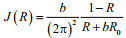

 (18)
(18)When R tends toward 0, the wave field will be unidirectional. This could lead to nonlinear focusing because of modulational instability, which raises the possibility of the formation of extreme waves. As R becomes larger (0 < R≤1), the sea state becomes multidirectional and the degree of focusing weakens. When R becomes larger than 1, the sea state will become defocused.
Another important parameter in the expression of C4dyn is the BFI. The BFI is the ratio of wave steepness to the spectral bandwidth in a unidirectional sea state, and it indicates the probability of occurrence of nonlinear focusing due to modulational instability. In deep water:
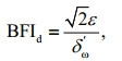 (19)
(19)where 
In the expression of C4dyn, the BFI2 should be considered with shallow water effects:
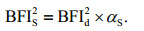 (20)
(20)In deep water αS=1, and as the depth limit k0d decreases, where k0 is the dominant wavenumber and d is the local depth, αS decreases slowly until k0d=1.363 and becomes negative, which means defocusing of nonlinear energy for k0d < 1.363 (Janssen and Onorato, 2007; Janssen and Bidlot, 2009). In this paper, we use the characteristic wave number k instead of k0.
3.4.5 Freakish sea indexAs indicated by the red stars in Fig. 9, none of the three rogue waves occurred at the "narrowest" moment. Affected by two wave systems with different wave directions, a slightly wider directional spreading is evidenced when events RW2215 and RW2222 occurred. In comparison with the other two events, it can be seen that event RW2106 has narrower directional spreading but the frequency bandwidth, indicated by Qp is not so narrow. The wide frequency bandwidth of all three events might be related to the stage of wave development. As discussed in Section 3.1, the wave field is quasi-fully developed when event RW2106 occurred, and the observation site was near the end of the wind fetch, which also had a fully developed sea state at the time the other two events occurred.

|
| Fig.9 Freakish sea index of events (a) RW2106 and (b) RW2215 and RW2222 |
The time evolutions of the degree of short crestedness and the irregularity parameters are shown in Fig. 10, in which the dashed lines indicate the times at which the rogue waves occurred. According to our simulated spectra at the observation site, the values of γs are 0.82, 0.85 and 0.81, indicating a higher degree of short crestedness of sea state at the times at which the rogue waves occurred. The irregularity parameter αxt is > 0.75 and the values of αyt and αxy are between 0.1–0.3, which indicate that the sea states were more organized along the direction of propagation and more confused along the y direction. For event RW2106, most wave energy was directed along the mean wave direction (toward WNW), which caused the confused wave field in the y direction. In events RW2215 and RW2222, the mean wave directions were toward N but the coexisting wave systems were toward NW and NE. The pair of opposite vector components toward W and E led to the confusion indicated by the low values of αyt and αxy.

|
| Fig.10 Degree of short crestedness and irregularity parameters |
From Eqs.11–14, we find λ3, NB and λ40, NB influenced primarily by wave steepness 

|
| Fig.11 Theoretical skewness and kurtosis in narrowband condition |
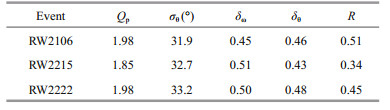
Figure 12 shows the time evolutions of envelope skewness and kurtosis. It can be seen that the values of C32 (black line) and C4 (green line) for event RW2106 are slightly larger than for events RW2215 and RW2222, which is consistent with our previous conclusions. It can also be found that the envelope kurtosis (green line) is dominated by the bound part (blue line), which contributes up to approximately 83%, 77% and 80% of the total C4 at the times at which the rogue wave events occurred. In comparison with the bound part, the dynamical envelope kurtosis (red line) is much smaller and the dynamical part in all three events is similar, denoting that even the narrower directional distribution in event RW2106 did not trigger active nonlinear focusing due to modulational instability. We show later that C3bound and C4bound are dominated primarily by wave steepness and that damping of wave steepness is caused by the degree of development of the waves. Many other factors contribute to C4dyn; however, despite the three peaks of C4dyn shown in Fig. 12, because no rogue wave was observed at the buoy at those moments, will do not discuss this further in this paper.

|
| Fig.12 Envelope skewness and kurtosis |
In Janssen (2018), R is shown affected by water depth. The time evolution of R with and without the effect of shallow water, and the relative directional and frequency width are all shown in Fig. 13. It can be seen that R decreased after the first event occurred (Fig. 13a), which led to a more unidirectional wave state (Fig. 13b). That decrease was caused by the widening of δω because of the increasingly developed sea state. However, parameter R is a ratio determined by both δω and δθ. Therefore, as another wave system was added, as concluded in Section 3.2, the relative directional width δθ became wider just before event RW2215 occurred. Thus, we observe an increase of R during the final two events, which means the sea state, became less unidirectional again.

|
| Fig.13 Parameter R and relative directional width (a) and frequency width (b) |
As shown in Fig. 14a, a damping trend of BFId can be seen from the time before event RW2106 occurred, except for a temporary "peak" due to a temporarily narrower δω', as shown in the top subplot in Fig. 14b. Several hours before event RW2215, the BFId started to increase again and it kept increasing gradually throughout the period during which events RW2215 and RW2222 occurred. Similar trends were noted in the evolutions of λ3, NB and λ40, NB in Fig. 11 and C3bound and C4bound in Fig. 12. Apparently, those parameters are all associated with wave steepness 

|
| Fig.14 Benjamin-Feir Index with shallow water effects |

|
| Fig.15 Wave steepness based on mean and characteristic wavenumber |
Greater damping of 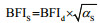
During August 2013, three rogue waves were recorded with an observation buoy deployed in the East China Sea at 29.068 7°N, 124.921 5°E. From the perspectives of wind and wave fields, wave system tracking, HOS method simulation, and characteristic parameters of sea state, we undertook a detailed analysis on three events using simulated results from the WAVEWATCH Ⅲ model. The principal conclusions are as follows.
1) All three rogue waves were influenced by Typhoon Trami (TY201312 CMA) but in different degrees. The sea state was quasi-fully developed and highly influenced by Trami when event RW2106 occurred. Then, as Trami made landfall and the storm became a tropical depression, weakening of Trami's influence was inevitable. After the storm made landfall and during the period when events RW2215 and RW2222 occurred, the local wind pattern changed at the observation site, which was located at the end of the local wind fetch.
2) The wave field was dominated completely by Typhoon Trami when event RW2106 occurred; thus, there was only one system in the wave field. Events RW2215 and RW2222 occurred as the storm diminished, which is when another system with a wave direction different to the local wind was added and became increasingly stable. According to the wave direction, the new system was probably generated by the southwest wind over the southern part of the East China Sea. Consequently, the directional distribution of event RW2106 was narrower than for the other two events.
3) All three events occurred in sea states dominated by second-order nonlinearities, and third-order quasi-resonant interactions were considered negligible in the formation of the rogue waves. Furthermore, the degree of nonlinearity was influenced primarily by wave steepness, which was closely associated with sea state development.
4) Modulational instability was considered negligible in the extreme events for three reasons. First, even with a narrower directional distribution, the fully or quasi-fully developed wind-generated waves broadened the frequency bandwidth in three events, i.e., the directional spectra had no chance to be "narrowest." Second, the damping of wave steepness reduced the BFI, which represents suppression of modulational instability; with a fully developed sea state and decreasing wind speed, such damping of wave steepness was unavoidable. Finally, shallow water effects dominated by the smaller wavenumber of a more developed sea state further stabilized the modulational instability. To conclude, the fully developed sea state suppressed the third-order quasi-resonant interactions and associated modulational instabilities.
The nonlinearities of sea state, which play an important role in the formation of rogue waves, are closely related to the degree of development of the waves. With the presence of a moving typhoon center, the development of the sea state becomes complex. The method adopted in this study can provide comprehensive and full-scale analysis of rogue waves in the real world. The case studied in this paper is not considered unique, and rules could be found and confirmed in relation to other typhoon sea states through the application of our proposed method.
5 DATA AVAILABILITY STATEMENTThe data that support the findings of this study are available on request from the corresponding author: JIANG Xingjie (jiangxj@fio.org.cn).
Ardhuin F, Rogers W, Babanin A V, Filipot J F, Magne R, Roland A, van der Westhuysen A, Queffeulou P, Lefevre J M, Aouf L, Collard F. 2010. Semiempirical dissipation source functions for ocean waves. Part Ⅰ:definition, calibration, and validation. J. Phys. Oceanogr., 40(9): 1917-1941.
DOI:10.1175/2010JPO4324.1 |
Barbariol F, Benetazzo A, Carniel S, Sclavo M. 2015. Spacetime wave extremes:the role of metocean forcings. J.Phys. Oceanogr., 45(7): 1897-1916.
DOI:10.1175/JPO-D-14-0232.1 |
Baxevani A, Rychlik I. 2006. Maxima for Gaussian seas. Ocean Eng., 33(7): 895-911.
DOI:10.1016/j.oceaneng.2005.06.006 |
Devaliere E M, Hanson J L, Luettich R. 2009. Spatial tracking of numerical wave model output using a spiral search algorithm. In: Proceedings of 2009 WRI World Congress on Computer Science and Information Engineering.IEEE, Angeles, CA, USA. p.404-408, https://doi.org/10.1109/CSIE.2009.1021.
|
Dommermuth D. 2000. The initialization of nonlinear waves using an adjustment scheme. Wave Motion, 32(4): 307-317.
DOI:10.1016/S0165-2125(00)00047-0 |
Dommermuth D G, Yue D K P. 1987. A high-order spectral method for the study of nonlinear gravity waves. J. Fluid Mech., 184: 267-288.
DOI:10.1017/S002211208700288X |
Ducrozet G, Bonnefoy F, Le Touzé D, Ferrant P. 2007. 3-D HOS simulations of extreme waves in open seas. Nat.Hazards Earth Syst. Sci., 7(1): 109-122.
DOI:10.5194/nhess-7-109-2007 |
Ducrozet G, Bonnefoy F, Le Touzé D, Ferrant P. 2016. HOSocean:open-source solver for nonlinear waves in open ocean based on high-order spectral method. Comput.Phys. Commun., 203: 245-254.
DOI:10.1016/j.cpc.2016.02.017 |
Ducrozet G, Bonnefoy F, Perignon Y. 2017. Applicability and limitations of highly non-linear potential flow solvers in the context of water waves. Ocean Eng., 142: 233-244.
DOI:10.1016/j.oceaneng.2017.07.003 |
Dysthe K, Krogstad H E, Müller P. 2008. Oceanic rogue waves. Annu. Rev. Fluid Mech., 40: 287-310.
DOI:10.1146/annurev.fluid.40.111406.102203 |
Dysthe K, Trulsen K, Krogstad H E, Socquet-Juglard H. 2003. Evolution of a narrow-band spectrum of random surface gravity waves. J. Fluid Mech., 478: 1-10.
DOI:10.1017/S0022112002002616 |
ECMWF. 2016. Part Ⅶ: ECMWF Wave Model. IFS Documentation CY43R1, https://www.ecmwf.int/node/17120.
|
Fedele F. 2008. Rogue waves in oceanic turbulence. Phys. D:Nonlinear Phenom., 237(14-17): 2127-2131.
DOI:10.1016/j.physd.2008.01.022 |
Fedele F. 2012. Space-time extremes in short-crested storm seas. J. Phys. Oceanogr., 42(9): 1601-1615.
DOI:10.1175/JPO-D-11-0179.1 |
Fedele F. 2015. On the kurtosis of deep-water gravity waves. J. Fluid Mech., 782: 25-36.
DOI:10.1017/jfm.2015.538 |
Fedele F, Brennan J, Ponce de León S, Dudley J, Dias F. 2016. Real world ocean rogue waves explained without the modulational instability. Sci. Rep., 6: 27715.
DOI:10.1038/srep27715 |
Fedele F, Lugni C, Chawla A. 2017. The sinking of the El Faro:predicting real world rogue waves during hurricane Joaquin. Sci. Rep., 7(1): 11188.
DOI:10.1038/s41598-017-11505-5 |
Fedele F, Tayfun M. 2009. On nonlinear wave groups and crest statistics. J. Fluid Mech., 620: 221-239.
DOI:10.1017/S0022112008004424 |
Fernandez L, Onorato M, Monbaliu J, Toffoli A. 2014. Modulational instability and wave amplification in finite water depth. Nat. Hazards Earth Syst. Sci., 14(3): 705-711.
DOI:10.5194/nhess-14-705-2014 |
Goda Y. 1970. Numerical experiments on wave statistics with spectral simulation. Rep. Port Harb. Res. Inst., 9(3): 3-57.
|
Hanson J L, Jensen R E. 2004. Wave system diagnostics for numerical wave models. In: Proceedings of the 8th International Workshop on Wave Hindcasting and Forecasting Turtle Bay Resort. Coastal and Hydraulics Laboratory, Oahu, Hawaii.
|
Hanson J L, Phillips O M. 2001. Automated analysis of ocean surface directional wave spectra. J. Atmos. Oceanic Technol., 18(2): 277-293.
DOI:10.1175/1520-0426(2001)018<0277:AAOOSD>2.0.CO |
Hanson J L, Tracy B A, Tolman H L, Scott R D. 2009. Pacific hindcast performance of three numerical wave models. J.Atmos. Oceanic Technol., 26(8): 1614-1633.
DOI:10.1175/2009JTECHO650.1 |
Hasselmann K. 1962. On the non-linear energy transfer in a gravity-wave spectrum part 1. General theory. J. Fluid Mech., 12(4): 481-500.
DOI:10.1017/S0022112062000373 |
Hasselmann K. 1963a. On the non-linear energy transfer in a gravity wave spectrum part 2. Conservation theorems; wave-particle analogy; irrevesibility. J. Fluid Mech., 15(2): 273-281.
DOI:10.1017/S0022112063000239 |
Hasselmann K. 1963b. On the non-linear energy transfer in a gravity-wave spectrum. Part 3. Evaluation of the energy flux and swell-sea interaction for a Neumann spectrum. J.Fluid Mech., 15(3): 385-398.
DOI:10.1017/S002211206300032X |
Hasselmann S, Hasselmann K, Allender J H, Barnett T P. 1985. Computations and parameterizations of the nonlinear energy transfer in a gravity-wave specturm. Part Ⅱ:parameterizations of the nonlinear energy transfer for application in wave models. J. Phys. Oceanogr., 15(11): 1378-1391.
DOI:10.1175/1520-0485(1985)015<1378:CAPOTN>2.0.CO;2 |
In K, Waseda T, Kiyomatsu K, Tamura H, Miyazawa Y, Iyama K. 2009. Analysis of a marine accident and freak wave prediction with an operational wave model. In: Proceedings of the 19th International Offshore and Polar Engineering Conference. SPE, Osaka, Japan. p.877-883.
|
Janssen P A E M. 2003. Nonlinear four-wave interactions and freak waves. J. Phys. Oceanogr., 33(4): 863-884.
DOI:10.1175/1520-0485(2003)33<863:NFIAFW>2.0.CO;2 |
Janssen P A E M. 2009. On some consequences of the canonical transformation in the Hamiltonian theory of water waves. J. Fluid Mech., 637: 1-44.
DOI:10.1017/S0022112009008131 |
Janssen P A E M. 2014. On a random time series analysis valid for arbitrary spectral shape. J. Fluid Mech., 759: 236-256.
DOI:10.1017/jfm.2014.565 |
Janssen P A E M. 2018. Shallow-water version of the Freak Wave Warning System. ECMWF Tech. Memo., 813.https://www.ecmwf.int/en/elibrary/18063-shallow-waterversion-freak-wave-warning-system.
|
Janssen P A E M, Bidlot J R. 2009. On the extension of the freak wave warning system and its verification. ECMWF Tech.Memo., 588. https://www.ecmwf.int/en/elibrary/10243-extension-freak-wave-warning-system-and-its-verification.
|
Janssen P A E M, Onorato M. 2007. The intermediate water depth limit of the zakharov equation and consequences for wave prediction. J. Phys. Oceanogr., 37: 2389-2400.
DOI:10.1175/JPO3128.1 |
Kharif C, Pelinovsky E. 2003. Physical mechanisms of the rogue wave phenomenon. Eur. J. Mech. B/Fluids, 22(6): 603-634.
DOI:10.1016/j.euromechflu.2003.09.002 |
Kharif C, Pelinovsky E, Slunyaev A. 2009. Rogue Waves in the Ocean. Springer, Berlin, Heidelberg, 2p. https://doi.org/10.1007/978-3-540-88419-4.
|
Kuik A J, van Vledder G P, Holthuijsen L H. 1988. A method for the routine analysis of pitch-and-roll buoy wave data. J. Phys. Oceanogr., 18(7): 1020-1034.
DOI:10.1175/1520-0485(1988)018<1020:AMFTRA>2.0.CO;2 |
Longuet-Higgins M S. 1957. The statistical analysis of a random, moving surface. Phil. Trans. Roy. Soc. A., 249(966): 321-387.
DOI:10.1098/rsta.1957.0002 |
Mori N, Janssen P A E M. 2006. On kurtosis and occurrence probability of freak waves. J. Phys. Oceanogr., 36(7): 1471-1483.
DOI:10.1175/JPO2922.1 |
Mori N, Onorato M, Janssen P A E M. 2011. On the estimation of the kurtosis in directional sea states for freak wave forecasting. J. Phys. Oceanogr., 41(8): 1484-1497.
DOI:10.1175/2011JPO4542.1 |
Pierson W J Jr, Moskowitz L. 1964. A proposed spectral form for fully developed wind seas based on the similarity theory of S. A. Kitaigorodskii. J. Geophys. Res., 69(24): 5181-5190.
DOI:10.1029/JZ069i024p05181 |
Saha S et al. 2011. NCEP Climate Forecast System Version 2(CFSv2) selected hourly time-series products. Research data archive at the national center for atmospheric research, computational and information systems laboratory, https://doi.org/10.5065/D6N877VB. Accessed 28 May 2018.
|
Sergeeva A, Slunyaev A. 2013. Rogue waves, rogue events and extreme wave kinematics in spatio-temporal fields of simulated sea states. Nat. Hazards Earth Syst. Sci., 13(7): 1759-1771.
DOI:10.5194/nhess-13-1759-2013 |
Tamura H, Waseda T, Miyazawa Y. 2009. Freakish sea state and swell-windsea coupling:numerical study of the Suwa-Maru incident. Geophys. Res. Lett., 36(1): L01607.
DOI:10.1029/2008GL036280 |
Tayfun M A. 1980. Narrow-band nonlinear sea waves. J.Geophys. Res. Oceans, 85(C3): 1548-1552.
DOI:10.1029/JC085iC03p01548 |
Tayfun M A. 2006. Statistics of nonlinear wave crests and groups. Ocean Eng., 33(11-12): 1589-1622.
DOI:10.1016/j.oceaneng.2005.10.007 |
Tayfun M A, Fedele F. 2007. Wave-height distributions and nonlinear effects. Ocean Eng., 34(11-12): 1631-1649.
DOI:10.1016/j.oceaneng.2006.11.006 |
Tayfun M A, Lo J M. 1990. Nonlinear effects on wave envelope and phase. J. Waterw. Port, Coastal, Ocean Eng., 116(1): 79-100.
DOI:10.1061/(ASCE)0733-950X(1990)116:1(79) |
The WAVEWATCH Ⅲ Development Group (WW3DG). 2016.User manual and system documentation of WAVEWATCH Ⅲ R Version 5.16. Tech. Note 329, NOAA/NWS/NCEP/MMAB, College Park, MD, USA, http://polar.ncep.noaa.gov/waves/WAVEWATCH/. Accessed 09 Mar 2018.
|
Toffoli A, Gramstad O, Trulsen K, Monbaliu J, Bitner-Gregersen E, Onorato M. 2010. Evolution of weakly nonlinear random directional waves:laboratory experiments and numerical simulations. J. Fluid Mech., 664: 313-336.
DOI:10.1017/S002211201000385X |
Tolman H L. 1991. A third-generation model for wind waves on slowly varying, unsteady, and inhomogeneous depths and currents. J. Phys. Oceanogr., 21(6): 782-797.
DOI:10.1175/1520-0485(1991)021<0782:ATGMFW>2.0.CO;2 |
Vincent L, Soille P. 1991. Watersheds in digital spaces:an efficient algorithm based on immersion simulations. IEEE Trans. Pattern Anal. Mach. Intell., 13(6): 583-598.
DOI:10.1109/34.87344 |
Voorrips A C, Makin V K, Hasselmann S. 1997. Assimilation of wave spectra from pitch-and-roll buoys in a North Sea wave model. J. Geophys. Res. Oceans, 102(C3): 5829-5849.
DOI:10.1029/96JC03242 |
Waseda T, Tamura H, Kinoshita T. 2012. Freakish sea index and sea states during ship accidents. J. Mar. Sci. Technol., 17(3): 305-314.
DOI:10.1007/s00773-012-0171-4 |
Waseda T, In K, Kiyomatsu K, Tamura H, Miyazawa Y, Iyama K. 2014. Predicting freakish sea state with an operational third-generation wave model. Nat. Hazards Earth Syst.Sci., 14(4): 945-957.
DOI:10.5194/nhess-14-945-2014 |
West B J, Brueckner K A, Janda R S, Milder D M, Milton R L. 1987. A new numerical method for surface hydrodynamics. J. Geophys. Res.:Oceans, 92(C11): 11803-11824.
DOI:10.1029/JC092iC11p11803 |
Xiao W T, Liu Y M, Wu G Y, Yue D K P. 2013. Rogue wave occurrence and dynamics by direct simulations of nonlinear wave-field evolution. J. Fluid Mech., 720: 357-392.
DOI:10.1017/jfm.2013.37 |
Ying M, Zhang W, Yu H, Lu X Q, Feng J X, Fan Y X, Zhu Y T, Chen D Q. 2014. An overview of the China meteorological administration tropical cyclone database. J. Atmos.Oceanic Technol., 31(2): 287-301.
DOI:10.1175/JTECH-D-12-00119.1 |
Zakharov V E. 1968. Stability of periodic waves of finite amplitude on the surface of a deep fluid. J. Appl. Mech.Tech. Phys., 9(2): 190-194.
DOI:10.1007/BF00913182 |