 2019, Vol. 37
Institute of Oceanology, Chinese Academy of Sciences
Article Information
- GUO Yunxia, HOU Yijun, QI Peng
- Analysis of typhoon wind hazard in Shenzhen City by Monte-Carlo Simulation
- Journal of Oceanology and Limnology, 37(6): 1994-2013
- http://dx.doi.org/10.1007/s00343-019-8231-9
Article History
- Received Sep. 7, 2018
- accepted in principle Dec. 6, 2018
- accepted for publication Feb. 28, 2019


2 University of Chinese Academy of Sciences, Beijing 100049, China;
3 Laboratory for Ocean and Climate Dynamics, Qingdao National Laboratory for Marine Science and Technology, Qingdao 266237, China;
4 Center for Ocean Mega-Science, Chinese Academy of Sciences, Qingdao 266071, China
Shenzhen City is located in the southeast coast of China with a highly developed economy and dense population and is one of the regions most seriously impacted by typhoons. Typhoon disasters have resulted in significant economic losses and heavy causalities in the southeast China coastal regions in history. It has been found that landfall of typhoons usually occurs in the southeast China coastal regions, including Shenzhen. In these areas, it is very important to analyze typhoon hazard risks and predict the design wind speeds of typhoons for the design of critical structures and typhoon disaster mitigation.
The design wind speeds and pressures given by current load code in China are obtained through statistically analyzing the measured wind data of the meteorological department. However, in the typhoonprone area, the anemometers are vulnerable to damage and the typhoon wind speed records are often too short, which all can lead to an inaccurate estimate of wind load. To solve the problem of lack of wind speed data, Monte-Carlo simulation as an alternative and feasible approach for typhoon wind hazard analysis is the most widely accepted. It uses the mature typhoon model and the typhoon history data to simulate the typhoon wind field and predict annual maximum wind speed. The United States (American Society of Civil Engineers, 2005) and Australia (SAA, 2002) use the method to compile the design wind speed maps.
Russell(1969, 1971) first described the simulation approach, and since that pioneering study, the modeling technique has been expanded and improved by others. Batts et al. (1980) and Shapiro (1983) successively developed the Batts hurricane model and Shapiro hurricane model. Georgiou (1986) proposed and developed the numerical simulation method about hurricane based on the Monte-Carlo method by statistically analyzing the hurricane history data combining the Georgiou typhoon model. Vickery and Twisdale (1995b) compared the Shapiro typhoon model and Batts model and indicated that the Shapiro model is better than the Batts model. Meng et al. (1995) investigated the wind field in a typhoon boundary layer known as Yan Meng (YM) typhoon model. Simiu and Scanlan (1996) reviewed the problems involved in the description of the wind climate for structural design purposes and in the development of criteria for the definition of design wind speeds. A procedure based on climatological and physical models of hurricanes were presented. Thompson and Cardone (1996) employed the numerical simulation method to hindcast the wind field of history hurricane cases in the Gulf of Mexico in order to obtain a series of extreme wind speeds. As indicated by Vickery and Twisdale (1995a), the approaches used in the previous studies are similar, with the major differences being associated with the filling models and wind field models. Other differences include the size of the region over which the typhoon climatology can be considered uniform and the use of a coast segment crossing approach (Russell, 1971; Batts et al., 1980) or a circular subregion approach (Georgiou et al., 1983; Georgiou, 1986; Neumann, 1991; Vickery and Twisdale, 1995a).
In 2000, Vickery et al. (2000b) developed a new simulation approach where the full track of a hurricane or tropical storm is modeled, which is also a pioneering study. After that, significant improvements have been made (Vickery et al., 2009). Vickery and Wadhera (2008) developed an updated statistical model for the Holland pressure profile parameter (B) and the radius to maximum winds (Rmax). This model was used by Li and Hong(2014, 2015, 2016) and Hong et al. (2016). Xiao et al. (2011) developed the empirical linear relation for lnRmax and lnB for 11 coastal cities of China based on the typhoons affecting the China coast region and some empirical information from other literature. Li and Hong (2015) indicated that the mean of B estimated by Xiao et al. (2011) is much greater than that predicted by Vickery and Wadhera (2008). Lin and Fang (2013) also indicated that the model given by Vickery and Wadhera (2008) is preferred. Zhao et al. (2013) developed Rmax and B model at sea level that is applicable for the Northwest Pacific Ocean. From the updated database, Fang et al.(2018a, b) updated the models. Vickery (2005) developed a new decay model for a hurricane. There have been other derivations of the full track method. Mudd et al. (2014) used the state-of-the-art hurricane prediction models to simulate hurricanes under IPCC climate change scenario RCP 8.5 for year 2100. Cui and Caracoglia (2016) assessed the lifetime costs of tall buildings from hurricane-induced damage based on the empirical track model along the US Atlantic coast in a warming climate. Lee and Rosowsky (2007) developed a framework to set up a hurricane wind speed database for the Northeast US coast under both the 2005 and future climate states. Rosowsky et al. (2016) updated the analysis performed by Mudd et al. (2014), because significant improvements have been made (Vickery et al., 2009).
Over the past several decades in China, there are many types of research on typhoon climates and typhoon effects on structures (Li et al., 1998, 2000, 2004). Generally, the super tall buildings or long-span bridges or nuclear plants require higher standards of safety, but there are no elaborate design wind speeds for these structures in the Chinese design code (Ministry of Housing and Urban-Rural Construction of the People's Republic of China, 2012). Thus, it is vital to develop a practical method for typhoon risk analysis in China coastal region. Chen (1981) and Sheng and Wu (1993) conducted much research on the wind field model. Chen (1992) obtained a new wind field model by analyzing the Rankine and Jelesnianski wind field models, and they corrected the defects of the two models. She et al. (1995) improved the CE (US Army Corps of Engineers) wind field model and established a dynamic boundary layer of the wind field model. Li and Duan (2005) simulated the typhoon Betty (87) and Weyne (86) by using the Shapiro wind field model and the simulated wind speeds agree well with the observations. Ou et al. (2002) did the research about typhoon risk analysis for key coastal cities in southeast China using the Batts et al. (1980) model. Zhao et al. (2005) combined the YM typhoon model and the Monte-Carlo simulation to optimize the values of typhoon parameters at Shanghai seashore. Tao et al. (2001) developed the probability distribution of annual typhoon maximum wind speed in Shanghai through the Monte-Carlo simulation. Xiao et al. (2011) conducted the typhoon wind hazard analysis for 11 major cities in the southeast China coastal regions combined the Thompson and Cardone (1996) typhoon model and the Monte-Carlo simulation. There is also some other research (Zhao et al., 2007; Xie, 2008; Wei, 2009; Xie et al., 2015) on the typhoon modeling and extreme value prediction for the coastlines of China.
In this study, typhoon hazard analysis was conducted for the coastal city of Shenzhen in southeastern China using a Monte-Carlo simulation that referred to the framework developed in previous work, e.g., Simiu and Scanlan (1996), Georgiou (1986), and Vickery and Twisdale(1995a, b). The primary source of data used for this study is the CMASTI (China Meteorological Administration-Shanghai Typhoon Institute) Best Track Dataset for Tropical Cyclones (TC) over the Western North Pacific (during 1949–2015). The data file contains the information of typhoon position and intensity in 6-h intervals including typhoon number and name, the position of typhoon center (longitude and latitude), central pressure, and 2-min mean maximum sustained wind near the TC center.
First, characteristic parameters (annual occurrence rate, central pressure deficit, translation speed, storm heading, and the minimum approach distance) of typhoons were extracted and their statistical distributions were established for Shenzhen by processing the data obtained from the China Meteorological Administration (CMA). Then, the Monte-Carlo method was employed to sample from each distribution to generate characteristic parameters of virtual typhoons. The sample size depends on the typhoon annual occurrence rate of Shenzhen and the total number of years for typhoons simulated (1 000- year in this paper). Subsequently, the Yan Meng (YM) wind field model and its solution scheme were introduced and the sensitivities of the wind field model to several parameters were discussed. Finally, the typhoon wind fields were calculated using the YM model and the extreme wind speeds for various return periods were predicted by extreme value distributions such as Weibull and Gumbel distributions.
There are some differences from previous studies and several aspects, which needs to be explained. Firstly, in this study, the Monte-Carlo simulation is adopted rather than the empirical track model developed by Vickery et al. (2000b) because we focus on the specific site rather than an extended region that could experience wind hazard due to the same typhoon events. Secondly, in many previous studies, the Shapiro (Simiu and Scanlan, 1996), Georgiou (Lee and Rosowsky, 2007; Mudd et al., 2014; Rosowsky et al., 2016) and Thompson & Gardone (Xiao et al., 2011) typhoon models are applied while there is little use of the YM typhoon model. The typhoon boundary layer of YM model is more physically meaningful than applying the empirical discount factor like Batts et al. (1980) and Georgiou et al. (1983) model. Besides, the YM model is simpler than the Thompson and Cardone (1996) model and accurate enough for typhoon simulation. Xie et al. (2014) compared the wind speeds calculated by YM model, CE model, and Shaprio model and found that the wind field simulated by YM model is in good agreement with the measured values. Li et al. (2009) also validated the efficiency of YM model for the Xiamen city. The YM model has been applied to the typhoon wind field model, such as Matsui et al. (2002), Xie et al. (2015). Therefore, we applied the YM wind field model in this study. Thirdly, since Xiao et al. (2011), several major typhoon events have occurred, which acts as an update to the typhoon dataset used by Xiao et al. (2011). Finally, while storm surge and flooding due to typhoons also cause damage, only the direct typhoon wind hazards (maximum wind speed) were considered herein. The Shenzhen City is selected as the case study; however, the framework can be applied in other typhoonaffected regions as well.
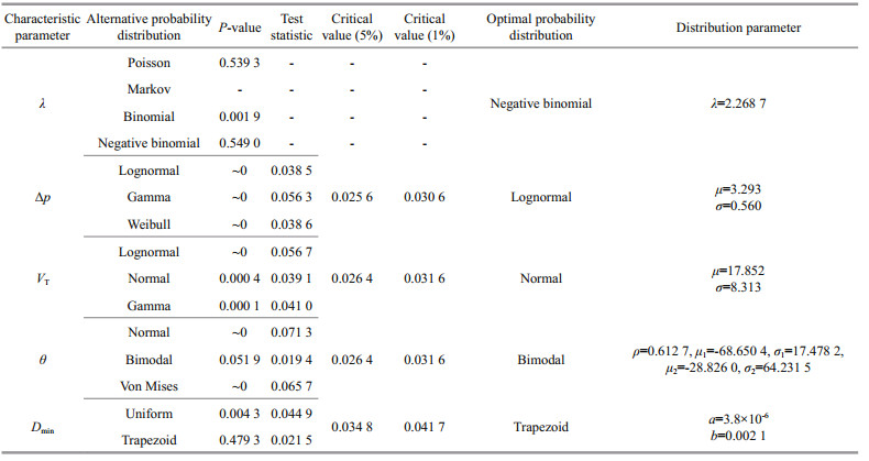
2 TYPHOON CHARACTERISTIC PARAMETER AND PROBABILITY DISTRIBUTIONA typhoon model is often parameterized by a set of parameters known as typhoon characteristic parameters: the annual occurrence rate, λ; central pressure deficit, Δp; radius to maximum winds, Rmax; translational speed, VT; storm heading, θ; and the minimum approach distance, Dmin. They are the variables that characterize the structure and intensity of a storm. The parameters are quantified by their probabilistic distributions, which can be determined based on publicly available records of historical typhoons. One sampling method used widely to establish the probabilistic distributions of typhoon characteristic parameters is to extract records of typhoon tracks that intersect and are within a simulation circle (given specified radius) centered at the site of interest. In this study, the simulation circle radius over which typhoon climatology could be considered uniform was set at 250 km. Alternative statistical probability distributions of typhoon characteristic parameters have been described by Vickery and Twisdale (1995a), Yasui et al. (2002), and Simiu and Scanlan (1996). In the current study, we used two nonparametric tests, i.e., the Chi-square test and the Kolmogorov-Smirnov test (KS test) to examine the goodness-of-fit of the statistical properties of the typhoon characteristic parameters. Finally, we derived the optimal probability model for each parameter for Shenzhen, which might be different from the Atlantic region. The results of the goodness-of-fit test for the typhoon characteristic parameters are presented in Table 1.
|
The annual occurrence rate for typhoons was derived from the frequency of typhoons within or passing through a circular sub-region centered on the site of interest. This is required to determine the size of sampling in the Monte-Carlo simulation. A probabilistic model of recurrence is usually described by a homogeneous (uniform) Poisson distribution, Markov chain model, binomial distribution, or negative binomial distribution. We examined all four probabilistic distributions for typhoon recurrence in Shenzhen and the results of the Chi-square test are displayed in Table 1. Figure 1 presents the modeled and observed statistical distributions of occurrence rate. Although the Markov chain model has better agreement with the observations, the probability of moving from one state to another is associated with the sample; therefore, if the sample lacks a corresponding occurrence number of typhoons, it will be neglected by the model, i.e., the model cannot predict a frequency that does not appear in the observation. It can be seen from the data in Table 1 that the binomial distribution does not pass the goodness-of-fit test and that the P-value of the negative binomial distribution is larger than that of the Poisson distribution. In China, the Poisson model is widely accepted as the simplest and robust model to describe the annual occurrence rate of typhoon events and the negative binomial distribution is nearly not examined. However, here we think the negative binomial distribution is superior to the Poisson distribution besides Vickery et al. (2000b) and Cui and Caracoglia (2015) suggested that a negative binomial distribution might be more appropriate. Therefore, this study adopted the negative binomial distribution to describe the annual occurrence rate of typhoon events.

|
| Fig.1 Modeled and observed statistical distributions of annual occurrence rate PMF (Probability Mass Function) is the probability of a discrete random variable. |
The central pressure deficit Δp is the difference between the central pressure and the periphery pressure (1 010.0 hpa for Northwest Pacific by Holland (1980)). It is an important parameter to describe the typhoon intensity and can be modeled using the lognormal, Gamma, or three-parameter Weibull distributions. Figure 2 shows the modeled and observed statistical distributions of central pressure deficit. The KS test was used to examine the goodness-of-fit of the three probabilistic distributions shown in Table 1. It can be seen that none of the three probabilistic distributions passed the KS test but the test statistic of the lognormal distribution was closest to the critical value, especially at the 1% significance level. Ou et al. (2002) indicated that when a test statistic is very close to the critical value, the distribution could be considered to have approximately passed the test. Therefore, we considered the lognormal distribution adequate for describing Δp.

|
| Fig.2 Modeled and observed statistical distributions of central pressure deficit |
The translation speed VT was derived from the 6-hourly position data of the typhoon center from the CMA dataset. The translation speed is calculated in the following form:
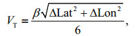 (1)
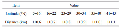
(1)where ΔLat is the latitude differences measured between two consecutive time instants (6 h), ΔLon is the longitude difference, and β is distance parameter related to the latitude, the values are given in Table 2.
The translation speed VT can be modeled using the lognormal, normal, or Gamma distributions. Figure 3 shows the modeled and observed statistical distributions of translation speed. The KS test was used to examine the goodness-of-fit of the three probabilistic distributions shown in Table 1. It can be seen that none of the three probabilistic distributions passed the KS test but the test statistic of normal distribution was closest to the critical value, especially at the 1% significance level. Therefore, we considered the normal distribution appropriate for describing the translation speed in this study.

|
| Fig.3 Modeled and observed statistical distributions of translation speed |
The storm heading θ represents the angle between the direction of translation and the true north and is positive for a clockwise angle. We examined the applicability of the normal, bimodal, and Von Mises distributions to represent the statistical characteristics of storm heading based on the KS test (Table 1). The bimodal distribution passed the KS test, even at the 5% significance level. Figure 4 shows the modeled and observed statistical distributions of storm heading. It is obvious that the bimodal distribution fits better than the other two probabilistic distributions. Therefore, the bimodal distribution was employed in this study.

|
| Fig.4 Modeled and observed statistical distributions of storm heading |
The minimum approach distance Dmin was the shortest distance from the typhoon track to the interest site and was defined as positive if the site of interest was located on the right side of the typhoon's translation direction. The minimum approach distance can be modeled using either a uniform or trapezoid distribution. Figure 5 shows the modeled and observed statistical distributions of minimum approach distance. Based on the goodness-of-fit test, the trapezoid distribution passed the KS test at the 5% significance level (Table 1). Therefore, the trapezoid distribution was used in this study to describe Dmin.

|
| Fig.5 Modeled and observed statistical distributions of minimum approach distance |
The radius to maximum winds Rmax is defined as the distance from the typhoon center to the region of maximum wind speed (Vickery et al., 2000b). In Vickery and Twisdale (1995a), two models were given for the radius to maximum winds as functions of latitude and central pressure. Later with the updated database, these models were also updated. For use in the storm track modeling approach, three new candidate global models for Rmax were developed by Vickery et al. (2000b). As an update, Vickery and Wadhera (2008) gave other two Rmax models, one for the Gulf of Mexico and one for all Atlantic Ocean. In China, given the absence of information on the Rmax in the historical records of the CMA, Rmax is usually derived using one of two methods. The first uses the radius to the wind speed of 10.8 m/s, i.e., the lower speed of Beaufort scale 6, referring to Li et al. (1995), while the other uses an empirical equation obtained following the approach of Vickery et al.(1995a, 2000b). The empirical equation, given by Jiang et al. (2008) based on the Tropical Cyclones Year Books of 1949–2002, is expressed as:
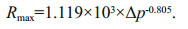 (2)
(2)Jiang et al. (2008) compared these two methods and obtained satisfactory results when calculating the wind field and wave field using Eq.2. They concluded the empirical equation was superior to the method proposed by Li et al. (1995). In this study, Eq.2 was adopted to describe the Rmax; however, we did not consider the effect of latitude on Rmax for three reasons. First, Eq.2 has been verified sufficiently accurate to describe Rmax by Jiang et al. (2008). Second, only a limited region of the southeast China coast (Shenzhen) was examined in this study. Third, referring to previous studies (Vickery and Twisdale, 1995a; Vickery and Wadhera, 2008), many models used to calculate Rmax are divided into two parts (i.e., south of 30°N and north of 30°N), and for storms located south of 30°N, latitude is not considered. Here, the area of focus of this study was the region located south of 30°N.
3 THE MONTE-CARLO SIMULATIONFor an analysis of typhoon wind risk, Monte-Carlo simulation is the most widely accepted as referred to Xiao et al. (2011). Reliability of the wind field model and the accuracy of the statistics for the typhoon characteristic parameters is the key to the success of the simulation.
3.1 Generating virtual typhoon seriesThe Monte-Carlo method was used to sample from each distribution of λ, θ, Dmin, VT, and Δp, as mentioned in Section 2, to generate the characteristic parameters of virtual typhoon genesis. This study simulated virtual typhoons for 1 000 years and the number of typhoons was determined by the annual occurrence rate distribution. By sampling 1 000 times from the distribution of annual occurrence rate, there are 2 199 virtual typhoons need to be generated. The samples of each characteristic parameter sampled from the optimal distribution are fitted by the optimal distribution again, and all of them pass the goodnessof-fit test at 95% confidence level. The steps adopted for the generation of the virtual typhoon series were as follows.
1) The characteristic parameters sampled from their probability distributions were constrained to the ranges of [0, 7] for λ, [0, 135] hpa for Δp, [2, 65] km/h for VT, [-180°, 180°] for θ, and ≤R (the radius of the simulation circle) for Dmin.
2) Using θ, Dmin, R, and the location of the simulation site to determine the genesis of the virtual typhoon, which is the intersection point of the typhoon track and simulation circle, as shown in Fig. 6.

|
| Fig.6 A schematic graph for simulation of the virtual typhoon SP: simulation point; LP: landing point; Dmin: minimum approach distance; R: radius of circular subregion; θ: storm heading. |
3) The track of the virtual typhoon was assumed a straight line in its evolution, and the values of θ and VT were used to obtain the typhoon center locations for each hour.
4) As a virtual typhoon moved ahead and made landfall on the coastline, a filling model was used to determine Δp.
5) The typhoon was assumed to move away from the simulation site when it passed beyond the simulation circle. A diagram of this procedure is shown in Fig. 6.
3.1.1 Fitting the coastlineIn the procedure of generating virtual typhoon, a coastline is needed to judge the typhoon's landfall place. The latitudes and longitudes of several cities along the southeast China coastal region were used to fit the coastline equation. Because the central locations of coastal cities are not near the sea, they were moved seaward by about 15–30 km to mark the intersection of the land and sea. The coastline was fitted using the polynomial shown in Eq.3 and as illustrated in Fig. 7:

|
| Fig.7 The fitting coastline |
 (3)
(3)where γ is the coastline longitude in degrees and ψ is the coastline latitude in degrees.
3.1.2 The filling modelWhen a typhoon makes landfall, its strength starts to decrease. Both the central pressure difference and the wind speed decrease according to some filling model. Batts et al. (1980), Georgiou (1986) and Vickery and Twisdale (1995b) define the rate of filling overland using the decay of the central pressure deficit, which is usually modeled as a function of either the time that has elapsed since the storm made landfall or the distance inland that the storm has traveled from the point at which it caused landfall. An exponential decay function developed by Vickery and Twisdale (1995b) is the most widely used. He developed three different filling model using central pressure and position data given in HURDAT (Hurricane Databases) for three geographical regions of the USA. This study employed a similar exponential model to describe typhoon decay for Shenzhen based on the CMA dataset.
The filling rate was modeled in the following form:
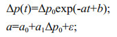 (4)
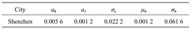
(4)where Δp(t) is the central pressure difference (hPa) at time t after landfall, Δp0 is the central pressure difference (hPa) at landfall, a is the decay constant, b is an error term assumed normally distributed with mean μb and standard deviation σb, and ε is a normally distributed error term with mean zero and standard deviation σε.
Eighty-four observed storms were used to develop a filling model for Shenzhen. The fitting curve of the exponential decay of the central pressure deficit for 12 storm cases is shown in Fig. 8. Figure 9 shows the fitted values of the decay constant (a) plotted versus the central pressure deficit at the time of landfall. Estimates of the coefficients for the filling model are given in Table 3.

|
| Fig.8 Exponential decay of central pressure deficit for 12 storms |

|
| Fig.9 Decay constant a versus the central pressure deficit at landfall SD: standard deviation. |
The wind field model is the key to the successful numerical simulation of a typhoon. The YM wind field model, proposed by Meng et al. (1995), was employed in this study. In order to evaluate the terrain roughness and topographical effect, the model involves the concept of the so-called "equivalent roughness length". The typhoon boundary layer of YM model is more physically meaningful than applying the empirical discount factor like Batts et al. (1980) and Georgiou et al. (1983) model. The complete analytical solution is derived through an intuitive solution of the gradient wind equation.
The Holland (1980) pressure model is used in this study:
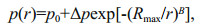 (5)
(5)where p(r) is the surface pressure at a distance r from the typhoon center, p0 is the central pressure, Δp is the central pressure deficit, B is the pressure profile constant, the range is estimated to be 0.5–2.5.
Considering that the strong wind field in a lower typhoon boundary layer is in a neutral condition (Meng et al., 1993), the equation of motion can be written as
 (6)
(6)where ρ is the air density, k is the vertical unit vector, f is the Coriolis parameter, V is the typhoon-induced wind velocity.
In the YM model, V is decomposed into the gradient wind Vg in the free atmosphere and the friction wind V′.
Since the pressure isobars in the domain of a moving typhoon are axisymmetric with respect to the center of the typhoon, the cylindrical coordinate system is used. The radial velocity Vrg can be obtained from the equation of continuity as follows,
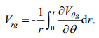 (7)
(7)Considering approximate accuracy, Vrg is set at 0 in the study of Meng et al. (1995).
Iterated computation is used to solve the YM wind field model. More details about the wind field model can be found in Meng et al. (1995).
4.2 Validation and sensitivity of the YM modelAmong the storms that have affected Guangdong Province in China, typhoon Hagupit (2008) was the most destructive, and it was used to validate the applicability of the YM model. Figure 10 shows the path of Typhoon Hagupit and the geographical locations of three marine meteorological stations: Shangchuandao (SCD), Yangjiang (YJ), and Dianbai (DB). The sensitivities of the YM wind field model to radial velocity Vrg, typhoon translation speed VT, radius to maximum winds Rmax, pressure profile constant B, and roughness length z0 are examined based on the measured data of Hagupit.

|
| Fig.10 Track of Typhoon Hagupit and geographical locations of three marine meteorological stations of Shangchuandao (SCD), Yangjiang (YJ), and Dianbai (DB) |
1) The sensitivity of radial velocity
Figure 11 shows the influence of Vrg=0 and 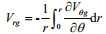


|
| Fig.11 Influence of Vrg on simulated wind speed and direction at station SCD |
2) The sensitivity of typhoon translation speed
Three methods were employed to determine the translation speed (VT) of Typhoon Hagupit to obtain different values of VT. Based on the measured location data of Typhoon Hagupit obtained from the Guangdong Meteorology Agency of China, Eq.1 or the toolbox of MATLAB (Matrix Laboratory, the 'distance' function in the map toolbox) can be used to calculate the translation speed, while the third method involves downloading the translation speeds directly from the Typhoon Network of China (2002). The calculated results of translation speed using method 1–3 are compared in Fig. 12 as vt1, vt2, and vt3, respectively. The translation speeds derived using the first two methods are similar and larger than that derived using the third method for most of the times. The effects of translation speed on the simulated wind speed and direction of Typhoon Hagupit at station SCD are illustrated in Fig. 13. It can be seen that the simulated wind speed increases slightly with increasing VT at every moment of the typhoon and VT has little influence on the simulated wind direction.

|
| Fig.12 The translation speeds calculated by three methods |

|
| Fig.13 Influences of VT on simulated wind speed and direction at station SCD |
3) The sensitivity of radius to maximum winds
In Section 2.6, several methods were introduced for the calculation of the radius to maximum winds (Rmax) and reasons for the adoption of the empirical equation derived by Jiang et al. (2008) were explained. Here, we examined the sensitivity of Rmax to the YM wind field model. Referring to previous studies, we adopted five different models to determine the radius to maximum winds:
(a) Single equation for Rmax was given by Vickery et al. (2000b):
lnRmax=2.63–0.00508Δp2+0.0394ψ;
(b) In Vickery and Wadhera (2008), two models were given for the Rmax, one for all hurricanes in Atlantic and one for Gulf of Mexico hurricanes, in which the Rmax was found to be independent of latitude. The model for the Gulf of Mexico is used in this study because we do not care much about the influence of latitude. The model is
lnRmax=3.859–7.7×10⁻⁵Δp2;
(c) The model fitted by Jiang et al. (2008) based on the data from Tropical Cyclones Year Books (1949–2002) is
Rmax=1.119×10³×Δp-0.805;
(d) The model fitted by Li (2007) for Guangdong province in China based on the least-square method is
lnRmax=-0.1239Δp0.6003+5.1034;
(e) The model proposed by Fang et al. (2018a) is
lnRmax=-38.36Δp0.025+46.75.
The Rmax values of Typhoon Hagupit calculated using the five models are different, as shown in Fig. 14. The effects of Rmax on the simulated wind speeds and directions of Typhoon Hagupit at station SCD are shown in Fig. 15. As can be seen in Fig. 15, changing Rmax has little effect on the maximum wind speed and it has virtually no effect on the wind direction for the example of station SCD located within about Rmax from the center of Hagupit. Vickery et al. (2000a) indicated that the effect of a change in Rmax varies depending on the position of the station relative to the center of the storm. For stations well beyond Rmax, increasing Rmax results in an increase in the simulated wind speed.

|
| Fig.14 The radius to maximum winds calculated by five different models |

|
| Fig.15 Influences of Rmax on simulated wind speed and direction at station SCD |
4) The sensitivity of pressure profile constant
The shape parameter of Holland pressure profile B is an important input parameter for the wind field model. At present, there is no uniformly accepted model for the calculation of B for typhoons affecting the coast of China. Referring to previous studies, this study considered nine different approaches for the calculation of B including eight models and a set of fixed values:
(a) The parameter B for typhoon Hagupit calculated by Xiao (2011);
(b) The Powell05 model (Powell et al., 2005): B=1.881–0.00557Rmax–0.01295ψ+ε;
(c) The Vickery08 model (Vickery and Wadhera, 2008): 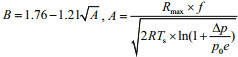
(d) The H & H99 model (Harper and Holland, 1999): B=2–(p0–900)/160;
(e) The Hubbert91 model (Hubbert et al., 1991): B=1.5+(980–p0)/120;
(f) The Jacboson model (Jakobsen and Madsen, 2004):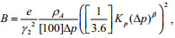
(g) The HAZUS-MH and HAZUS-MH MR1 Hurricane Model User Manual (National Institute of Building Science, 2009) (Federal Emergency Management Agency, FEMA): B=1.38+0.00184Δp–0.00309Rmax;
(h) The Fang model (Fang et al., 2018a):
B=4.1025×10⁻⁵×Δp2+0.0293×Δp+0.7959×ln(Rmax)–4.6010;
(i) A set of fixed values: B=0.4, 0.6, 0.8, 1.0, 1.2, 1.4. The B values of Typhoon Hagupit calculated using the eight models (a–h) show the considerable difference (Fig. 16). The effects of B calculated using the eight models on the simulated wind speed and direction at station SCD are shown in Fig. 17. Figure 18 is the same as Fig. 17, except B is set to fixed values. The simulated wind speed is very sensitive to changes in B, as can be seen in Figs. 17 & 18. An increase in B results in an increase in the maximum storm wind speed. Vickery et al. (2000a) indicated that changing B has an effect on the simulated maximum wind speed at each station and that the impact varies depending on the position of the station relative to the storm center. The B values calculated using the first seven models are generally larger than 1.2 and for the Typhoon Hagupit, these B values may be too large. Thus, the simulated maximum wind speeds are also overestimated as shown in Fig. 17 and the maximum relative difference between the simulated and observed maximum wind speed is up to 50%. The simulated wind speeds calculated by the eighth model are in the best agreement with the measured values among the eight models. For the fixed values of B, when the B value is about 0.8, the simulated wind speed can agree well with the observed winds. Xie (2008) also found that when the value of B is around 0.9, the simulated wind speed agrees well with the measured values for the YM model.

|
| Fig.16 The pressure profile parameter calculated by the first eight models |

|
| Fig.17 Influences of B calculated by the first eight models on the simulated wind speed and direction at station SCD |

|
| Fig.18 Influences of fixed values of B on the simulated wind speed and direction at station SCD |
5) The sensitivity of the roughness length
The YM wind field model introduces the concept of "equivalent roughness length" to simulate the boundary layer profile. The roughness length (z0) is also very important for the typhoon wind field model. Generally, the roughness length is small for flat open terrain and large for rough areas. The effects of different roughness length values (z0=0.005 m, 0.01 m, 0.02 m, 0.05 m, 0.1 m, 0.2 m, and 0.5 m) on simulated wind speed and direction were investigated in this study, as shown in Fig. 19. The simulated wind speed decreases substantially with increasing roughness length, and the simulated wind direction also varies with z0. Therefore, the simulated wind speed is very sensitive to changes in z0. As long as the value of z0 is reasonable, the simulated wind speed and direction can match the measured values reasonably well.

|
| Fig.19 Influences of z0 on the simulated wind speed and direction at station SCD |
The effects of the pressure profile constant B and roughness length z0 on the simulated wind speed and direction were also examined for stations YJ and DB. The adoption of reasonable values of B and z0 resulted in a reasonable agreement between the simulated results and the observations, as shown in Figs. 20 & 21, validating the applicability of the YM wind field model to the region of the southeast coast of China.

|
| Fig.20 Measured and simulated wind speed and direction of Typhoon Hagupit at station YJ |

|
| Fig.21 Measured and simulated wind speed and direction of Typhoon Hagupit at station DB |
Based on the probability models of typhoon characteristic parameters in Section 2, virtual typhoon series obtained by Monte-Carlo simulation in Section 3, and the YM wind field model in Section 4, the extreme wind speed series was calculated. For Shenzhen City, we generated 2 199 virtual typhoons by Monte-Carlo simulation. In addition, the YM model was used to calculate the wind speed of each virtual typhoon. We extracted the maximum wind speed of each typhoon to form the extreme wind speed series. Theoretical probabilistic distributions are often used to model the extreme wind speed series. The widely used Gumbel and Weibull distributions were employed in this study and tested through the goodness-of-fit KS test. We predicted wind speeds with different return periods for Shenzhen to provide references for the design wind speed, wind resistance, and disaster mitigation.
The sensitivity analyses of the wind field parameters described earlier indicated that B and z0 are both very important to the wind field model. The smaller the B value is, the lower the simulated wind speed is, and the smaller z0 is, the higher the simulated wind speed is. For improved simulation of the actual wind field in different regions, the values of B and z0 were determined by minimizing the deviation between the simulated maximum wind speed and the measured maximum wind speed. Here, we considered the ranges of z0 and B as 0.05–2.0 and 0.6–2.0, respectively. The 1 000-year simulated typhoons were substituted into the YM model under different combinations of B and z0 to calculate their respective maximum wind speed at the national basic meteorological station of Shenzhen. Then, the simulated respective maximum wind speed under different combinations of B and z0 was compared with the measured maximum wind speed in Shenzhen over the past 60 years. The deviation of the simulated maximum wind speed under the different combinations of B and z0 from the measured maximum wind speed is shown in Fig. 22. It is clear from Fig. 22 that when B increases linearly with z0, the deviation of the simulated maximum speed from the measured maximum wind is smallest. This is because increasing B makes the simulated maximum speed larger than the measured value, whereas increasing z0 makes the simulated maximum speed smaller than the measured value. Therefore, when B and z0 increase simultaneously, the simulated maximum wind speed can agree well with the measured value. Consequently, the smallest deviations of the simulated maximum wind speed from the measured maximum wind speed are distributed along the diagonal line in Fig. 22.

|
| Fig.22 Deviation of the simulated maximum wind speed under different combinations of values of B and z0 from the measured maximum wind speed |
Based on Monte-Carlo simulation, the sample of extreme wind speed with a capacity of m is obtained. The typhoon hazard is defined as the probability P that the wind speed V caused by typhoon exceeds the threshold vi, within a given time t.
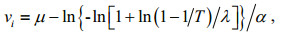
For the empirical distribution (or sample distribution), the derived wind speed of return period T is
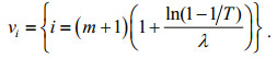 (8)
(8)The formula in curly braces is the calculation for subscript i. When the sample of wind speed is arranged from small to large, i is the rank of the extreme wind speed for a return period of T.
For the Weibull distribution, the derived wind speed of return period T is
 (9)
(9)where β is the shape parameter; η is the scale parameter; and γ is the location parameter.
For the Gumbel distribution, the derived wind speed of return period T is
 (10)
(10)where μ is the location parameter and α is the scale parameter.
The Chinese design code (Ministry of Housing and Urban-Rural Construction of the People's Republic of China, 2012) specifies the design wind pressures of different return periods (10, 50 and 100 years) in B terrain for the Guangzhou, Hong Kong, Shenzhen, and Xiamen, etc. That is shown in Table 4. The code also gives the transformation formula of design wind pressure for other return periods:

 (11)
(11)where XT is the design wind pressure of T years return period. The relation between design wind speed v0 and the design wind pressure ω0 given by the code is
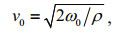 (12)
(12)where ρ is the air density, ρ=0.001 25 e-0.001Z, and Z is the altitude of Shenzhen City.
5.2 Extreme wind speed estimation for different return periodsThe Chinese design code (Ministry of Housing and Urban-Rural Construction of the People's Republic of China, 2012) gives the recommended 10-min average wind speed at the 10-m level for B terrain. Therefore, this study predicted wind speed under the same conditions. A conversion factor of 1.06 was employed to convert the simulated 1-h average wind speeds to 10-min average wind speeds.
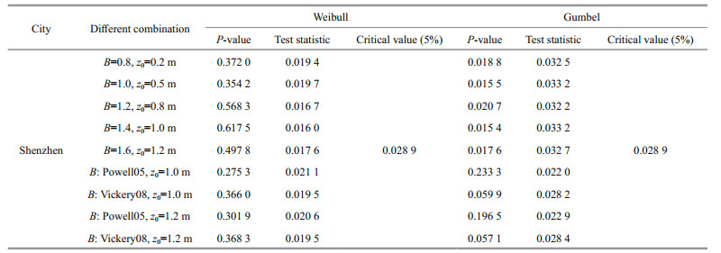
The estimated parameters of extreme value distributions under the different combinations of B and z0, corresponding to the small deviations in Fig. 22, are presented in Table 5. The KS test at the 5% significance level was used to examine the goodnessof-fit of the Weibull and Gumbel distributions, as shown in Table 6. It can be seen that under the different combinations of B and z0 Weibull distribution pass the significance test. As determined by the P-values, the Weibull distribution is better suited than the Gumbel distribution to describe extreme wind speed. The Chinese design code (Ministry of Housing and UrbanRural Construction of the People's Republic of China, 2012) recommends the Gumbel distribution for extreme wind speed estimation; however, we suggest the extreme value distribution should be chosen according to the actual situation.

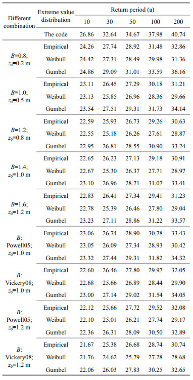
The empirical, Weibull, and Gumbel distributions were used to predict extreme wind speeds for different return periods. Table 7 shows the 10-min average extreme wind speeds for different return periods at the 10-m level under different combinations of values of B and z0.
|
Taking the results of the 100-year return period as an example, the predicted extreme wind speeds using different extreme value distributions under different combinations of values of B and z0 are compared in Fig. 23.

|
| Fig.23 The predicted extreme wind speed of the 100-year return period |
It can be seen from Table 7 and Fig. 23 that the predicted extreme wind speeds based on the Weibull distribution are generally lower than from the empirical distribution. Moreover, the predicted extreme wind speeds based on the Gumbel distribution are generally higher than from the empirical distribution. The simulated extreme wind speeds for different return periods are smaller than recommended in the structural code under the listed combinations of values of B and z0. As determined in Fig. 23, when B=0.8 and z0=0.2 m, the predicted extreme wind speed is highest. With further increases in the values of B and z0, the predicted extreme wind speed first decreases and then increases slightly for all three extreme value distributions. This is because when B is small, z0 plays a leading role in decreasing the predicted extreme wind speed. Conversely, when B is large, B plays a leading role in increasing the predicted extreme wind speed.
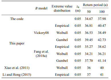
For comparison purpose, we list the predicted extreme wind speeds of 50-year and 100-year return periods for Shenzhen City from Xiao et al. (2011) and Li and Hong (2015) by using Monte-Carlo simulation, as shown in Table 8. As indicated by Li and Hong (2015) the Chinese code (Ministry of Housing and Urban-Rural Construction of the People's Republic of China, 2012) suggests z0=0.05 m for the standard site condition B. Thus they set z0 to 0.05 m and they converted the values of Xiao et al. (2011) to those for z0=0.05 m. The values of Li and Hong (2015) in Table 8 are obtained using the Lognormal distribution for Δp and in this paper, the Δp is also fitted by Lognormal distribution. For consistency, we also predict the wind speeds of 50-year and 100-year return periods for Shenzhen City when z0 is set to 0.05 m and B is calculated by Vickery08 and Fang model (Fang et al., 2018a) and the results are shown in Table 8. It can be seen from Table 8 that the results predicted by empirical distribution in this paper are similar to those of Xiao et al. (2011) and Li and Hong (2015), and all the predicted results are about 5% larger than those from the design code. The predicted wind speeds by Fang model are generally smaller than those from the Vickery08 model because the B values calculated by Fang model are smaller than those from the Vickery08 model seen from Fig. 16.
|
It can be seen from the above analysis that the prediction of extreme wind speed is very sensitive to z0 and B. z0 can be obtained according to the actual topography. The difficulty of prediction lies in the determination of B value. Due to the lack of observational typhoon data, there is no more accurate scheme to calculate B in China currently. Therefore, we can only use the different calculation schemes of B to predict the extreme wind speed for reference.
6 CONCLUSIONThe typhoon wind hazard risk for Shenzhen was analyzed using a Monte-Carlo simulation and the YM wind field model. Based on historical typhoon records and optimal statistical distributions for the typhoon characteristic parameters, the Monte-Carlo simulation generated 2199 virtual typhoon events for a 1 000- year period. The wind fields of these virtual typhoons were simulated using the YM wind field model. Extreme wind speeds for various return periods were predicted using the structural code and the empirical, Weibull, and Gumbel distributions. Based on the findings, we suggested the extreme value distribution should be chosen according to the actual situation.
Sensitivities of the YM model to radial velocity, typhoon translation speed, and radius to maximum winds, pressure profile constant, and the roughness length were discussed in detail. While consideration of the radial velocity has almost no effect on the simulated wind speed, the simulated wind speed increases slightly with increasing translation speed at every moment of the typhoon. Changing the radius to maximum winds has little effect on the maximum wind speed and it has virtually no effect on the wind direction in cases where the site of interest is located within about Rmax from the center of the typhoon. An increase in B results in an increase in the maximum storm wind speed. Simulated maximum wind speeds are overestimated when adopting the value of B calculated using any of the first seven models considered in this study. In addition, the wind speeds from Fang model agree best with the measured results. The simulated wind speed decreases significantly with increasing roughness length. It is concluded that the YM model is very sensitive to changes in the values of B and z0. Parameters B and z0 have opposite effects on the simulated wind speeds; when B increases with increasing z0, the deviation of the simulated from the measured maximum wind speed is smallest.
This study considered the coastal city of Shenzhen as a point. Substituting a point for an area in an analysis of the typhoon wind hazard will unavoidably miss some significant extreme wind speeds. On occasion, this error might be substantial; therefore, the regional typhoon risk should be studied in the future.
7 DATA AVAILABILITY STATEMENTThe observed typhoon data that support the findings of this study are available in the CMA-repository (http://tcdata.typhoon.org.cn). The datasets generated during the current study are available from the corresponding author on reasonable request.
8 ACKNOWLEDGMENTData from the CMA-STI Best Track Dataset for Tropical Cyclones over the Western North Pacific online dataset are gratefully acknowledged. Thanks are extended to the reviewers.
American Society of Civil Engineers. 2005. ASCE/SEI 7-05 minimum design loads for buildings and other structures. ASCE, US.
|
Batts M E, Simiu E, Russell L R. 1980. Hurricane wind speeds in the United States. Journal of the Structural Division, 106(10): 2001-2016.
|
Chen K M. 1981. The typhoon pressure field and wind field models. Acta Oceanologica Sinica, 3(1): 44-56.
(in Chinese with English abstract) |
Chen K M. 1992. A new method calculating typhoon wind field. Marine Forecasts, 9(3): 60-65.
(in Chinese with English abstract) |
Cui W, Caracoglia L. 2015. Simulation and analysis of intervention costs due to wind-induced damage on tall buildings. Engineering Structures, 87: 183-197.
DOI:10.1016/j.engstruct.2015.01.001 |
Cui W, Caracoglia L. 2016. Exploring hurricane wind speed along US Atlantic coast in warming climate and effects on predictions of structural damage and intervention costs. Engineering Structures, 122: 209-225.
DOI:10.1016/j.engstruct.2016.05.003 |
Fang G S, Zhao L, Cao S Y, Ge Y J, Pang W C. 2018a. A novel analytical model for wind field simulation under typhoon boundary layer considering multi-field correlation and height-dependency. Journal of Wind Engineering and Industrial Aerodynamics, 175: 77-89.
DOI:10.1016/j.jweia.2018.01.019 |
Fang G S, Zhao L, Song L L, Liang X D, Zhu L D, Cao S Y, Ge Y J. 2018b. Reconstruction of radial parametric pressure field near ground surface of landing typhoons in Northwest Pacific Ocean. Journal of Wind Engineering and Industrial Aerodynamics, 183: 223-234.
DOI:10.1016/j.jweia.2018.10.020 |
Georgiou P N, Davenport A G, Vickery B J. 1983. Design wind speeds in regions dominated by tropical cyclones. Journal of Wind Engineering and Industrial Aerodynamics, 13(1-3): 139-152.
DOI:10.1016/0167-6105(83)90136-8 |
Georgiou PN. 1986. Design Wind Speeds in Tropical Cyclone-Prone Regions. University of Western Ontario, London, Canada.
|
Harper B A, Holland G J. 1999. An updated parametric model of the tropical cyclone. In: Proceedings of the 23rd Conference on Hurricanes and Tropical Meteorology. AMS, Dallas, Texas.
|
Holland G J. 1980. An analytic model of the wind and pressure profiles in hurricanes. Monthly Weather Review, 108(8): 1212-1218.
DOI:10.1175/1520-0493(1980)108<1212:AAMOTW>2.0.CO;2 |
Hong H P, Li S H, Duan Z D. 2016. Typhoon wind hazard estimation and mapping for coastal region in mainland China. Natural Hazards Review, 17(2): 04016001.
DOI:10.1061/(ASCE)NH.1527-6996.0000210 |
Hubbert G D, Holland G J, Leslie L M, Manton M J. 1991. A real-time system for forecasting tropical cyclone storm surges. Weather and Forecasting, 6(1): 86-97.
DOI:10.1175/1520-0434(1991)006<0086:ARTSFF>2.0.CO;2 |
Jakobsen F, Madsen H. 2004. Comparison and further development of parametric tropical cyclone models for storm surge modelling. Journal of Wind Engineering and Industrial Aerodynamics, 92(5): 375-391.
DOI:10.1016/j.jweia.2004.01.003 |
Jiang Z H, Hua F, Qu P. 2008. A new scheme for adjusting the tropical cyclone parameters. Advances in Marine Science, 26(1): 1-7.
(in Chinese with English abstract) |
Lee K H, Rosowsky D V. 2007. Synthetic hurricane wind speed records: development of a database for hazard analyses and risk studies. Natural Hazards Review, 8(2): 23-34.
DOI:10.1061/(ASCE)1527-6988(2007)8:2(23) |
Li Q S, Fang J Q, Jeary A P, Wong C K, Liu D K. 2000. Evaluation of wind effects on a supertall building based on full-scale measurements. Earthquake Engineering & Structural Dynamics, 29(12): 1845-1862.
|
Li Q S, Fang J Q, Jeary A P, Wong C K. 1998. Full scale measurements of wind effects on tall buildings. Journal of Wind Engineering and Industrial Aerodynamics, 74-76: 741-750.
DOI:10.1016/S0167-6105(98)00067-1 |
Li Q S, Xiao Y Q, Wong C K, Jeary A P. 2004. Field measurements of typhoon effects on a super tall building. Engineering Structures, 26(2): 233-244.
DOI:10.1016/j.engstruct.2003.09.013 |
Li Q, Duan Z D. 2005. Shapiro typhoon wind-field model and its numerical simulation. Journal of Natural Disasters, 14(1): 45-52.
(in Chinese with English abstract) |
Li R L. 2007. Prediction of Typhoon Extreme Wind Speeds based on Improved Typhoon Key Parameters. Harbin Institute of Technolog, Harbin, China. (in Chinese with English abstract)
|
Li S H, Hong H P. 2014. Observations on a hurricane wind hazard model used to map extreme hurricane wind speed. Journal of Structural Engineering, 141(10): 04014238.
|
Li S H, Hong H P. 2015. Use of historical best track data to estimate typhoon wind hazard at selected sites in China. Natural Hazards, 76(2): 1395-1414.
DOI:10.1007/s11069-014-1555-z |
Li S H, Hong H P. 2016. Typhoon wind hazard estimation for China using an empirical track model. Natural Hazards, 82(2): 1009-1029.
DOI:10.1007/s11069-016-2231-2 |
Li T, Lei Y, Xu Z Q, Liu C. 2009. Initiative research on typhoon simulation by YanMeng wind field model. Journal of Xiamen University (Natural Science), 48(6): 840-843.
(in Chinese with English abstract) |
Li X L, Pan Z D, She J. 1995. A method for adjustment of typhoon parameters. Journal of Oceanography of Huanghai & Bohai Seas, 13(2): 11-15.
(in Chinese with English abstract) |
Lin W, Fang W H. 2013. Regional characteristics of Holland B parameter in typhoon wind field model for Northwest Pacific. Tropical Geography, 33(2): 124-132.
(in Chinese with English abstract) |
Matsui M, Ishihara T, Hibi K. 2002. Directional characteristics of probability distribution of extreme wind speeds by typhoon simulation. Journal of Wind Engineering and Industrial Aerodynamics, 90(12-15): 1541-1553.
DOI:10.1016/S0167-6105(02)00269-6 |
Meng Y, Matsui M, Hibi K. 1993. A theoretical analysis of the wind field in the typhoon boundary layer. Journal of Wind Engineering, 55: 7-8.
|
Meng Y, Matsui M, Hibi K. 1995. An analytical model for simulation of the wind field in a typhoon boundary layer. Journal of Wind Engineering and Industrial Aerodynamics, 56(2-3): 291-310.
DOI:10.1016/0167-6105(94)00014-5 |
Ministry of Housing and Urban-Rural Construction of the People's Republic of China. 2012. GB 50009-2012 Load code for the design of building structures. Construction Industry Press of China, Beijing. (in Chinese)
|
Mudd L, Wang Y, Letchford C, Rosowsky D. 2014. Assessing climate change impact on the U.S. east coast hurricane hazard: temperature, frequency, and track. Natural Hazards Review, 15(3): 04014001.
DOI:10.1061/(ASCE)NH.1527-6996.0000128 |
National Institute of Building Science. 2009. HAZUS-MH MR4 hurricane model technical manual. Federal Emergency Management Agency.
|
Neumann C J. 1987. The National Hurricane Center Risk Analysis Program (HURISK). NOAA Tech. Memo. NWS-NHC-38, U.S. Department of Commerce, National Oceanic and Atmospheric Administration, National Hurricane Center, Miami.
|
Ou J P, Duan Z D, Chang L. 2002. Typhoon risk analysis for key coastal cities in southeast China. Journal of Natural Disasters, 11(4): 9-17.
(in Chinese with English abstract) |
Powell M, Soukup G, Cocke S, Gulati S, Morisseau-Leroy N, Hamid S, Dorst N, Axe L. 2005. State of Florida hurricane loss projection model: atmospheric science component. Journal of Wind Engineering and Industrial Aerodynamics, 93(8): 651-674.
DOI:10.1016/j.jweia.2005.05.008 |
Rosowsky D V. Mudd L, Letchford C. 2016. Assessing climate change impact on the joint wind-rain hurricane hazard for the northeastern U.S. coastline. In: Gardoni P, Murphy C, Rowell A eds. Risk Analysis of Natural Hazards: Interdisciplinary Challenges and Integrated Solutions. Springer, Cham. p. 79-92.
|
Russell L B. 1969. Probability Distributions for Texas Gulf Coast Hurricane Effects of Engineering Interest. Stanford University, Stanford.
|
Russell L R. 1971. Probability distributions for hurricane effects. Journal of the Waterways, Harbors and Coastal Engineering Division, 97(1): 139-154.
|
Shapiro L J. 1983. The Asymmetric boundary layer flow under a translating hurricane. Journal of the Atmospheric Sciences, 40(8): 1984-1998.
DOI:10.1175/1520-0469(1983)040<1984:TABLFU>2.0.CO;2 |
She J, Yuan Y L, Pan Z D. 1995. Numerical model of the typhoon wind field over the sea surface and its hindcast calibration. Acta Oceanologica Sinica, 17(3): 24-31.
(in Chinese) |
Sheng L F, Wu Z M. 1993. A new fitting method for sea surface wind field of typhoon. Journal of Tropical Meteorology, 9(3): 265-271.
(in Chinese with English abstract) |
Simiu E, Scanlan R H. 1996. Wind Effects on Structures: Fundamentals and Applications to Design. John Wiley & Sons, Inc., New York.
|
Standards Association of Australia. 2002. AS/NZS 1170.2: 2002 structural design actions part2: wind actions. Standards Association of Australia, New Zealand.
|
Tao L Y, Yan J Y, Xu J L. 2001. Application of Monte-Carlo simulation method in wind engineering. Journal of Nanjing Institute of Meteorology, 24(3): 410-414.
(in Chinese with English abstract) |
Thompson E F, Cardone V J. 1996. Practical modeling of hurricane surface wind fields. Journal of Waterway, Port, Coastal, and Ocean Engineering, 122(4): 195-205.
DOI:10.1061/(ASCE)0733-950X(1996)122:4(195) |
Typhoon Network of China. 2002. http://www.typhoon.org.cn/. Accessed on 2002-03-01. (in Chinese)
|
Vickery P J, Skerlj P F, Steckley A C, Twisdale L A. 2000a. Hurricane wind field model for use in hurricane simulations. Journal of Structural Engineering, 126(10): 1203-1221.
DOI:10.1061/(ASCE)0733-9445(2000)126:10(1203) |
Vickery P J, Skerlj P F, Twisdale L A. 2000b. Simulation of hurricane risk in the U.S. using empirical track model. Journal of Structural Engineering, 126(10): 1222-1237.
DOI:10.1061/(ASCE)0733-9445(2000)126:10(1222) |
Vickery P J, Twisdale L A. 1995a. Prediction of hurricane wind speeds in the United States. Journal of Structural Engineering, 121(11): 1691-1699.
DOI:10.1061/(ASCE)0733-9445(1995)121:11(1691) |
Vickery P J, Twisdale L A. 1995b. Wind-field and filling models for hurricane wind-speed predictions. Journal of Structural Engineering, 121(11): 1700-1709.
DOI:10.1061/(ASCE)0733-9445(1995)121:11(1700) |
Vickery P J, Wadhera D, Twisdale L A, Lavelle F M. 2009. U.S. hurricane wind speed risk and uncertainty. Journal of Structural Engineering, 135(3): 301-320.
|
Vickery P J, Wadhera D. 2008. Statistical models of Holland pressure profile parameter and radius to maximum winds of hurricanes from flight-level pressure and H*Wind data. Journal of Applied Meteorology and Climatology, 47(10): 2497-2517.
DOI:10.1175/2008JAMC1837.1 |
Vickery P J. 2005. Simple empirical models for estimating the increase in the central pressure of tropical cyclones after landfall along the coastline of the United States. Journal of Applied Meteorology, 44(12): 1807-1826.
DOI:10.1175/JAM2310.1 |
Wei W. 2009. Typhoon Wind Hazard Analysis of Shenzhen based on Wind-Field Model Numerical Simulation. Harbin Institute of Technology, Shenzhen. (in Chinese with English abstract)
|
Xiao Y F, Duan Z D, Xiao Y Q, Ou J P, Chang L, Li Q S. 2011. Typhoon wind hazard analysis for southeast China coastal regions. Structural Safety, 33(4-5): 286-295.
DOI:10.1016/j.strusafe.2011.04.003 |
Xiao Y F. 2011. Typhoon wind hazard analysis based on numerical simulation and fragility of light-gauge steel structure in southeast China coastal regions. Harbin Institute of Technology, Harbin, China. (in Chinese with English abstract)
|
Xie R Q, Li X L, Wang Y H, Fang D X. 2015. Typhoon wind numerical simulation and hazard analysis for Guangdong Province. Journal of Anhui Jianzhu University, 23(4): 51-55.
(in Chinese with English abstract) |
Xie R Q, Wu T, Wang Y H. 2014. Adaptability research on typhoon wind-field model. Journal of Hefei University (Natural Sciences), 24(2): 84-88.
(in Chinese with English abstract) |
Xie R Q. 2008. Numerical simulation and typhoon wind hazard analysis based on CE wind-field model and Yan Meng wind-field mode. Harbin Institute of Technology, Harbin, China. (in Chinese with English abstract)
|
Yasui H, Ohkuma T, Marukawa H, Katagiri J. 2002. Study on evaluation time in typhoon simulation based on Monte Carlo method. Journal of Wind Engineering and Industrial Aerodynamics, 90(12-15): 1529-1540.
DOI:10.1016/S0167-6105(02)00268-4 |
Zhao L, Ge Y J, Song L L, Mao H Q. 2007. Monte-Carlo simulation analysis of typhoon extreme value wind characteristics in Guangzhou. Journal of Tongji University (Natural Science), 35(8): 1034-1038.
(in Chinese with English abstract) |
Zhao L, Ge Y J, Xiang H F. 2005. Application of typhoon stochastic simulation and its extreme value wind prediction. Journal of Tongji University (Natural Science), 33(7): 885-889.
(in Chinese with English abstract) |
Zhao L, Lu A P, Zhu L D, Cao S Y, Ge Y J. 2013. Radial pressure profile of typhoon field near ground surface observed by distributed meteorologic stations. Journal of Wind Engineering and Industrial Aerodynamics, 122: 105-112.
DOI:10.1016/j.jweia.2013.07.009 |