 2020, Vol. 38
Institute of Oceanology, Chinese Academy of Sciences
Article Information
- GAO Yongli, MU Mu, ZHANG Kun
- Impacts of parameter uncertainties on deep chlorophyll maximum simulation revealed by the CNOP-P approach
- Journal of Oceanology and Limnology, 38(5): 1382-1393
- http://dx.doi.org/10.1007/s00343-020-0020-y
Article History
- Received Jan. 13, 2020
- accepted in principle Feb. 21, 2020
- accepted for publication Apr. 3, 2020


2 University of Chinese Academy of Sciences, Beijing 100049, China;
3 College of Science, China University of Petroleum(East China), Qingdao 266580, China;
4 Institute of Atmospheric Sciences, Fudan University, Shanghai 200433, China;
5 Qingdao National Laboratory for Marine Science and Technology, Qingdao 266237, China;
6 Center for Ocean Mega-Science, Chinese Academy of Sciences, Qingdao 266071, China
The deep chlorophyll maximum (DCM) is a subsurface peak in chlorophyll a, and refers to the equilibrium of phytoplankton growth with opposing resource gradients, including light from the surface and nutrients from below (Huisman et al., 2006; Harrison and Smith, 2011). The DCM is a widespread ecological phenomenon that exists in most oceans and lakes (Fee, 1976; Barbiero and Tuchman, 2001). Previous studies have demonstrated that the DCM has a close relationship with climate processes (Boyce et al., 2010; Doney et al., 2012), biogeochemical cycles (Brandini et al., 2014; Laufkötter et al., 2015), and particularly the carbon cycle (Paquette and Beisner, 2018). To understand the dynamics of DCM formation, numerical models describing marine ecosystems have been widely used (e.g., Christian et al., 2002; Heinle and Slawig, 2013).
Ocean ecosystem models usually involve multiple parameters that represent various physical and biochemical processes (Fulton et al., 2003; Kantha, 2004). The uncertainties of these parameters are primary sources of discrepancies between modeled DCM and observations (Losa et al., 2004). However, accurate estimates of these parameters are challenging due to the following reasons. First, parameters that contribute to ocean ecosystem simulations tend to change under different environmental conditions (Yoshiyama et al., 2009). For example, although there are many different phytoplankton species in the ocean ecosystem, the parameters associated with these species are commonly set as constants. Furthermore, it is unrealistic to expect to improve the accuracy of all parameters by field observations because of the large number of uncertain parameters and the high cost of ocean observations. Therefore, it is necessary to identify important parameters (i.e. sensitive parameters) that cause relatively large simulation or prediction errors. Improving these priority parameters can lead to better simulations or predictions of the ocean ecosystem.
To-date, there have been many proposed approaches to identify sensitive parameters. Specifically, some of them employ the data assimilation technique (e.g., Fiechter, 2012; Weir et al., 2013; Schartau et al., 2017). This strategy seeks to minimize the difference between temporally varying modeled and observed data by adjusting the value of control parameters. For instance, Evensen et al. (1998) constructed a penalty function for estimating poorly known parameters and found this method was only feasible for problems involving weak nonlinearity. Fennel et al. (2001) estimated parameter sensitivity based on posterior errors built with a Hessian matrix. Their study emphasized the importance of parameter optimization in testing the reliability of dynamic models. In contrast to data assimilation, some other approaches employ a variance-based methodology (Saltelli et al., 2005; Chu et al., 2007). This strategy tries to identify sensitive parameters by assessing their contribution to output variability. By utilizing special metrics of warping functions and irreversible predictability, Chu et al. (2007) explored the nonlinear sensitivity of model outputs to parameters and found this strategy feasible for parameters with an extremely wide range. Nonetheless, this approach requires a large quantity of computing resources, especially to investigate the sensitivities of multiple parameters. In recent years, Mu et al. (2010) proposed a new approach, conditional nonlinear optimal perturbation related to parameters (CNOP-P), to investigate the impact of parameter uncertainties with a nonlinear regime. The CNOP-P approach seeks to find the most sensitive parameter or parameter combination that induces the largest effect on simulating/predicting investigated events. This approach saves computing power and simultaneously considers nonlinear interactions among different parameters. To-date, the CNOP-P approach has been successfully utilized in parameter sensitivity analyses of net primary productivity in eastern China (Sun and Mu, 2014), predictions of soil carbon (Sun and Mu, 2017), and double-gyre variations (Yuan et al., 2019).
In this study, we investigated parameter sensitivity on simulating the DCM using the CNOP-P approach. By employing a nutrients-phytoplankton ecosystem model, we first identified the sensitivity of each parameter and then investigated the sensitivity of combinations that involves different parameters. The rest of this paper is organized as follows. A brief description of the nutrients-phytoplankton ecosystem model and the CNOP-P approach are presented in Section 2. Sensitivity studies of single parameter and parameter combination are discussed in Section 3. The improvements in the DCM simulation caused by reducing parameter uncertainties are presented in Section 4. Finally, Section 5 presents the summary and discussion.
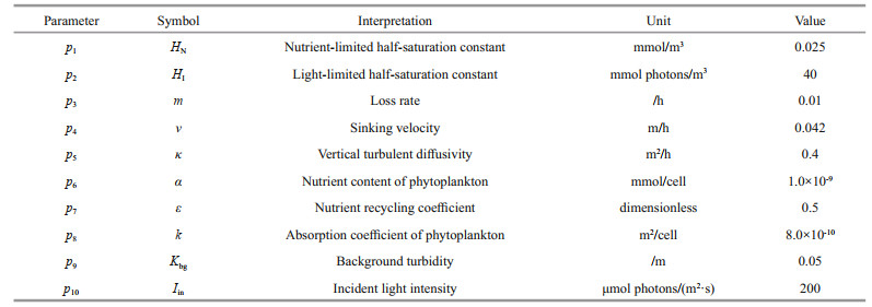
2 MODEL AND APPROACH 2.1 A nutrients-phytoplankton ecosystem modelIn this paper, the DCM was simulated by a onedimensional ecosystem model, which is able to reproduce most ecological features in the upper ocean (e.g., Huisman et al., 2006; Löptien, 2011; Liccardo et al., 2013). This model describes phytoplankton and nutrient dynamics limited by the supply of light and nutrients. The governing equations of phytoplankton Ph (cells/m3) and nutrients N (mmol/m3) are given by:
 (1)
(1)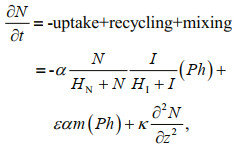 (2)
(2)where z is the water depth, t is the integration time, m is the loss rate of phytoplankton, κ is the coefficient of vertical turbulent diffusivity, α is the nutrient content of phytoplankton, ε is the nutrient recycling coefficient, ν is the phytoplankton sinking velocity; I is light intensity; and HN and HI are the half-saturation constants for nutrient-limited and light-limited growth, respectively.
Due to attenuation from concentrated phytoplankton and background turbidity, incident light intensity decreases with water depth. Using Lambert-Beer's equation (Kirk, 1994), the expression for the incident light intensity can be written as
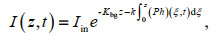 (3)
(3)where Iin is the incident light intensity at the top of the water column; k and Kbg are the attenuation coefficients of background turbidity and concentrated phytoplankton, respectively. As shown in Table 1, the values of all parameters are consistent with previous studies (Liccardo et al., 2013; Wang and Mu, 2015).
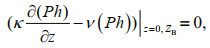
Regarding boundary conditions, the fluxes of phytoplankton and nutrients are
 (4)
(4) (5)
(5)where ZB denotes the bottom of the water column.
By employing a forward difference scheme, we discretized Eqs.1 & 2 in resolution of 0.5 m (600 vertical grids in total) and integrated the model for 20 years with a time step of 0.01 h. As the depleted nutrients and attenuated light for phytoplankton growth achieve a balance below the surface (Fig. 1a & b), the system gradually reaches a stable DCM equilibrium. We present the vertical nutrient and phytoplankton profiles of the 20th year in Fig. 1c & d. The maximum phytoplankton biomass is located at ~85 m, consistent with observational results and model simulations (Navarro and Ruiz, 2013; Wang and Mu, 2015).

|
| Fig.1 Temporal and spatial evolutions of profiles for equilibrium solutions a. nutrients (mmol/m3); b. phytoplankton (×108 cells/m3); c. vertical nutrients; d. phytoplankton. |
Mu et al. (2010) proposed the CNOP-P to investigate the effects of uncertainties of single parameter and parameter combination consisting of multiple parameters. In this study, the optimal single parameter or parameter combination revealed by the CNOP-Ps is regarded as the most sensitive parameter(s), which leads to maximal uncertainty in numerical simulations. The detailed derivation of the CNOP-P approach is introduced next.
A general nonlinear evolution equation can be expressed as
 (6)
(6)where t represents time and F is a nonlinear propagator. U∈Rn is the state variable, U0 is its initial value, and p=(p1, p2, p3, ∙∙∙, pn) is the vector consisting of all model parameters. Let Mt be the nonlinear propagator of the differential equations from the initial time 0 to t, then U(t)= Mt(U0, p) is the solution of Eq.6 at time t. U(t; U0, p) and U(t; U0, p)+u(t; U0, p′) are the solutions for vectors p and p+p′, where u(t; U0, p′) represents the departure from the reference state U(t; U0, p) caused by parameter perturbation p′. They satisfy the following equations
 (7)
(7)For a given norm ||•||, a parameter perturbation pΩ′ is called a CNOP-P if and only if
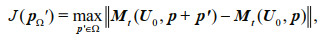 (8)
(8)where J is the cost function and Ω is the constraint of parameter perturbation. Essentially, CNOP-P (pΩ′) is the optimal parameter perturbation causing the largest variation of the cost function.
2.2.2 Settings for calculating the CNOP-PIn this study, the parameter vector consists of 10 parameters (Table 1). These parameters are related to major biological and physical processes, including nutrient (p1) and light (p2, p8, p9, p10) limitations that affect the growth of phytoplankton, loss of phytoplankton from death (p3) and gravity (p4), turbulent mixing of water (p5), and internal nutrient supply (p6, p7). We denote them in a vector p=(p1, p2, p3, ∙∙∙, p10). Previous studies have shown that phytoplankton biomass is a good proxy for DCM intensity (Klausmeier and Litchman, 2001; Wang and Mu, 2015). Thus, the objective function which is employed to seek the maximal change in DCM intensity is defined as
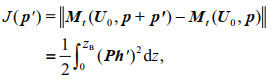 (9)
(9)where ||•|| is the L2 norm and Ph′ is the change in phytoplankton caused by parameter perturbation p′. In addition, the equilibrium of nutrients and phytoplankton presented in Fig. 1c & d is taken as the reference state to calculate the CNOP-P. The optimization time (t=1 080 d) was selected based on the diffusive timescale (Beckmann and Hense, 2007; Wang and Mu, 2015). This optimization time can ensure the ecosystem reaches a new equilibrium after the model is superimposed with parameter perturbations. We also verified that the parameter sensitivity results remain unchanged when the optimization time is changed to 720 d or 1 440 d. In addition, the differential evolution optimization algorithm, which displays strong global convergence and robustness (Storn and Price, 1997), is used to obtain the CNOP-P.
3 SENSITIVITY ANALYSIS OF SINGLE PARAMETER AND MULTIPLE PARAMETERS 3.1 Sensitivity analysis of single parameterFor each of the 10 selected parameters, we use the CNOP-P approach to calculate its optimal perturbation and examine its impacts on DCM simulations. Specifically, we employ pi′ to denote the perturbation of pi. To examine whether the sensitivity of single parameter depends on the constraint of parameter perturbation, different constraint values are selected with the following equation
 (10)
(10)where λ is the factor modulating the amplitude of perturbation constraint. To ensure a reasonable DCM position of 50–100 m (e.g., Huisman et al., 2006; Liccardo et al., 2013), λ≤0.4 is selected. Moreover, different values of λ, which ranges from 0.1 to 0.4 at an interval of 0.1, are used to explore the impacts of different perturbation constraints on the CNOP-P calculations. Hence, to study the sensitivity under different constraints, four different optimization experiments are conducted for each parameter.
Figure 2 demonstrates the sensitivity of the 10 parameters according to the cost function values caused by the CNOP-Ps. For different constraints, the parameter sensitivity rankings are similar. Moreover, the CNOP-P for each parameter is located at the boundary of the perturbation constraint. Here, we focus on the four most sensitive parameters since they induce relatively large changes in the DCM. The sensitivity ranking among the four most sensitive parameters basically remains unchanged for different parameter perturbation constraints. The most sensitive parameter is always p9 (Kbg, background turbidity), which limits light supply in the model. The corresponding cost function value is more than four times as large as the average caused by the CNOP-Ps related to the other parameters. Furthermore, p6 (α, nutrient content of phytoplankton), p7 (ε, nutrient recycling coefficient), and p5 (κ, vertical turbulent diffusivity) are the other three most sensitive parameters. The cost function values caused by the CNOP-Ps of these three parameters are about three times as large as the average caused by the six nonsensitive parameters.

|
| Fig.2 Cost function values caused by the CNOP-Ps related to single parameter under various perturbation constraints for λ=0.1 (a); λ=0.2 (b); λ=0.3 (c); λ=0.4 (d) X-axis labels denote the sequence number of selected parameters (see Table 1). |
Parameter p9 affects the light supply from the surface, whereas the other three sensitive parameters are related to nutrient supply. Therefore, superimposing these parameter perturbations affects the DCM equilibrium between light and nutrient supplies. To investigate how these four sensitive parameters specifically affect the DCM, the DCM changes caused by superimposing the CNOP-Ps of the sensitive parameters were examined. For brevity, only the CNOP-Ps obtained with λ=0.3 are discussed here, which induce corresponding perturbations of p9′=-0.015, p6′=-3.0×10¹⁰, p7′=0.15, and p5′=0.12.
Reduced background turbidity (p9′) allows light to reach deeper into the water column, leading to the rapid phytoplankton growth and biomass increase in the lower euphotic zone. At the same time, phytoplankton consumes more nutrients and thereby limits the phytoplankton growth in the upper layer (Fig. 3a & e). Eventually, a one-third increase in phytoplankton biomass and a deeper DCM are found after integration of 360 d (Fig. 3i). Additionally, the enhanced vertical turbulent diffusivity (p5′) and nutrient recycling coefficient (p7′) both increase the nutrient supply (Fig. 3g & h). The decline in the nutrient content of phytoplankton (p6′) indirectly results in a greater nutrient supply because each cell requires less nutrients under this condition (Fig. 3f). The abundant nutrient supply first benefits the phytoplankton growth in the upper euphotic zone (Fig. 3b–d). The concentrated phytoplankton in the upper water column subsequently prevents light penetration, further leading to a decrease in phytoplankton in the lower euphotic zone. This results in intensified and shallower DCMs (Fig. 3j–l).

|
| Fig.3 Temporal and spatial evolutions of phytoplankton (×108 cells/m3; a, b, c, d), and nutrient (mmol/m3; e, f, g, h) changes by separately superimposing the CNOP-P of parameter p9, p6, p7, and p5; and the corresponding vertical profiles of phytoplankton after integration of 360 d (i, j, k, l) The dotted lines in i, j, k, and l represent the phytoplankton vertical profiles in the reference state. |
Despite the analysis of single parameter sensitivities, it is important to remember that in ocean ecosystem models, the physical and biological processes represented by various parameters do not exist independently. Interactions among parameters play an important role in the identification of sensitive parameters (Chu et al., 2007; Sun and Mu, 2016; Wang et al., 2017). Thus, in this study, the impacts of multiple parameter perturbations on DCM simulations are further investigated by calculating the CNOP-Ps of parameter combinations.
Studies on parameter combinations can reflect the interactions among multiple parameters. Particularly, we aim to figure out whether the optimal parameter combination is a simple combination of the top four sensitive parameters (p5, p6, p7, p9). If yes, are their CNOP-Ps the same to those obtained from the single parameter analysis? If not, how do the interactions among various parameters affect the identification of sensitive parameters? To answer these questions, we examined the sensitivity of 210 (C104) groups of parameter combinations. Note that only the perturbation constraint of λ=0.3 is investigated for brevity. In addition, we have verified that the most sensitive parameter combination does not change at λ=0.1, 0.2, and 0.4. Furthermore, 16 CNOP-Ps of parameter combinations do not reach the perturbation constraint boundaries. This may be attributed to the nonlinear interactions among different parameters in a combination.
Figure 4 demonstrates the cost function values caused by the CNOP-Ps of the 210 groups of parameter combinations. The maximum cost function value occurs when the parameter combination of (p3, p5, p6, p7) is perturbed. It is nearly 2.5 times as large as the average caused by the CNOP-Ps of all parameter combinations. It is noted that the optimal parameter combination is different with (p5, p6, p7, p9). The cost function caused by the perturbation of (p5, p6, p7, p9) only shows the 13th largest value. Except for p3 (m, rate of phytoplankton loss) and p9, the other three parameters (p6, p7, p9) are the same in these two combinations.

|
| Fig.4 Cost function values caused by the CNOP-Ps related to parameter combinations under the perturbation constraint of λ=0.3 |
To further validate the importance of p3, Table 2 lists the frequency of each parameter in the 10 most sensitive combinations. We found that p3 occurs eight times, whereas p9 only occurs twice. Thus, p3 plays an important role in the identification of sensitive parameter combinations. However, with regard to single parameter sensitivity, p9 is the most sensitive and p3 is not sensitive at all (Fig. 2). This raised the question why p3 displays such importance in the optimal parameter combination. Are the nonlinear interactions among different parameters responsible for this?

To answer these questions, we superimposed the CNOP-P of the optimal parameter combination (p3′=-0.003, p5′=0.12, p6′=-3.0×10⁻¹⁰, p7′=0.15) where p3′ represents a decrease in the rate of phytoplankton loss, leading to an increase in phytoplankton. The nutrient supply is essential to maintain this significant increase. In this case, p5′, p6′, and p7′ provide abundant nutrients, as discussed in Section 3.1. Overall, these four types of perturbations eventually lead to nutrient increases (Fig. 5c), which results in increased phytoplankton biomass and a shallower DCM (Fig. 5a & e). However, no additional nutrients are provided when only p3 is perturbed. Therefore, p3 is not sensitive as a single parameter.

|
| Fig.5 Temporal and spatial evolutions of phytoplankton (×108 cells/m3; a, b) and nutrient (mmol/m3; c, d) changes after superimposing the CNOP-Ps of parameter combinations (p3, p5, p6, p7) and (p5, p6, p7, p9); the corresponding vertical profiles of phytoplankton after integration of 360 d (e, f) The dotted lines in i, j, k, and l represent the phytoplankton vertical profiles in the reference state. |
In contrast, p9 shows less sensitivity in the sensitivity analysis of multiple parameters. The optimal perturbation (p5′=0.12, p6′=-3.0×10⁻¹⁰, p7′=0.15, and p9′=-0.005 66) was superimposed on the reference state. The influence of p9′ on the DCM is opposite to the other three parameters (Fig. 3a). Specifically, p9′ induces a deeper DCM, whereas the DCM moves to a shallower depth with p5′, p6′, and p7′. Therefore, there is an opposite effect when the model is simultaneously perturbed with p5′, p6′, p7′, and p9′. As such, phytoplankton showed less of an increase compared with that caused by the optimal perturbation combination (p3′=-0.003, p5′=0.12, p6′=-3.0×10⁻¹⁰, p7′=0.15) and p9 shows less sensitivity (Fig. 5b & f).
The interactions among different parameters present a remarkable influence on the identification of sensitive parameters. For the ocean ecosystem, there are effects that enhance and cancel the physical and biological processes represented by different parameters. The sensitivity analysis of single parameter only evaluates the importance of one parameter and so cannot consider enhancement or cancellation effects. In contrast, the sensitivity analysis of multiple parameters with the CNOP-P approach can reflect different physical or biological processes (especially important processes) at the same time. Hence, sensitive parameters identified by the CNOP-Ps of parameter combinations should be more effective at improving the performance of DCM simulations.
4 IMPACT OF REDUCING PARAMETER UNCERTAINTIESOne of the most important objectives in identifying sensitive parameters is to reduce the uncertainties in numerical simulations or predictions. Errors in sensitive parameters are expected to be corrected through observations or laboratory experiments. Thus, we investigated whether DCM simulations can be significantly improved by eliminating uncertainties in sensitive parameters. Specifically, the sensitive parameters identified in the sensitivity analyses of single parameter and multiple parameters are examined, respectively.
In most cases, we are most concerned about parameter perturbations that can lead to large uncertainties in numerical simulations (Sun and Mu, 2016). Thus, using the same perturbation constraint (λ=0.3), the CNOP-P of the 10 parameters was calculated. As a result, pall′=(-0.007 5, -12, -0.003, -0.012 6, 0.12, -3.0×10¹⁰, 0.15, -2.4×10¹⁰, 0.006 652, 60) was obtained, which lead to the largest DCM simulation errors. The uncertainties of the sensitive parameters, identified by the CNOP-Ps of single and multiple parameters, were reduced based on pall′. Specifically, the uncertainties of the parameters p3, p5, p6, and p7, identified with the optimal parameter combination, were first reduced by utilizing the controlling factor δ1 defined in Eq.11.2 (denoted as pcase1′). For comparison, we also reduced the uncertainties in the other two parameter combinations (denoted as pcase2′ and pcase3′). According to δ2 (Eq.11.3), pcase2′ reduces uncertainties of the four sensitive parameters obtained from the single parameter analysis. Additionally, pcase3′ reduces the uncertainties of the remaining parameters, except for the optimal parameter combination, controlled by δ3 (Eq.11.4).
The improvement extent τ for uncertainties in DCM simulations is quantified by
 (11.1)
 (11.2)
 (11.3)
 (11.4)
where μ is the ratio modulating the extent of reductions of parameter perturbation (varying from 0.1 to 0.4 at an interval of 0.1) and integration of t=360 d.
Figure 6 illustrates the improvements in DCM simulations after reducing the uncertainties of the three groups of parameters. Better DCM simulations were consistently achieved with larger values of μ. However, for different values of μ, reducing perturbations of p1, p2, p4, p8, p9, and p10 produced no significant improvements. This indirectly reflects the importance of identifying sensitive parameters by the CNOP-P approach because most of these six parameters are not included in the CNOP-Ps of either sensitive single or multiple parameters. More importantly, for cases with the same value of μ, reducing parameter errors from the most sensitive parameter combination (p3, p5, p6, p7) always produces the best model performance. For different values of μ, improvements in reducing perturbations from the most sensitive parameter combination are 10%–25% better than those caused by the sensitive parameters p5, p6, p7, and p9. In particular, when μ is 0.4, the improvement induced by this group of parameters achieves a high value (~76%). Therefore, focusing on sensitive parameters identified by CNOP-P of single and, especially, multiple parameters is very effective in improving DCM simulations.

|
| Fig.6 Improvements in DCM simulations by reducing uncertainties of the three parameter-groups The yellow, blue, and red bars indicate improvements by reducing parameter uncertainties in pcase1′, pcase2′ and pcase3′, respectively. |
Using a nutrients-phytoplankton ecosystem model and the CNOP-P approach, this study explored the impacts of parameter uncertainties on simulating the DCM. First, the DCM was successfully simulated by the ocean ecosystem model. Then, the sensitivity of single parameter was investigated by calculating the CNOP-Ps related to 10 individual parameters. A sensitivity ranking of the 10 parameters was obtained according to the cost function values caused by the CNOP-Ps. The top four sensitive parameters were further analyzed because they were shown to induce relatively large changes in the DCM. Specifically, the most sensitive single parameter is p9 (Kbg, background turbidity). The CNOP-P of p9 enhances the light supply for the ecosystem, and thereby leads to increased phytoplankton and a deeper DCM. The other three sensitive parameters are p6 (α, nutrient content of phytoplankton), p7 (ε, nutrient recycling coefficient), and p5 (κ, vertical turbulent diffusivity). By enhancing the nutrient supply, the CNOP-Ps of these three parameters all lead to increases in phytoplankton and upward moves of the DCM.
Considering the importance of interactions among different parameters, the sensitivity of multiple parameters was further investigated by calculating the CNOP-Ps related to combinations of four parameters. As a result, the optimal parameter combination (p3, p5, p6, p7) was identified. Interestingly, the parameters in the optimal parameter combination are not the same as the top four sensitive parameters obtained from the single parameter analysis. In the optimal parameter combination, p9 is replaced by p3 (m, loss rate). Further investigation indicates p3 becomes more important because of the abundant nutrient supply caused by perturbations of p5, p6, and p7. In contrast, there is a cancellation effect between the perturbation of p9 and the other three parameters. This cancellation effect also limits p9′ to a boundary value.
Finally, we quantified the improvement in DCM simulations by reducing the uncertainties of the identified sensitive parameters. Compared with nonsensitive parameters, reducing uncertainties of the sensitive parameters always exhibit better performances. Moreover, the sensitive parameters in the optimal parameter combination are more effective than those obtained from the single parameter analysis. This again emphasizes the importance and necessity of considering the interactions of various parameters for parameter sensitivity analysis.
The CNOP-P approach is effective in identifying sensitive single parameters and parameter combinations. Our results highlight the importance of considering interactions among different parameters for the identification of sensitive parameters. The CNOP-P approach related to parameter combination can identify sensitive parameters more effectively, especially for models that involve a large number of parameters. Reducing the uncertainties of these sensitive parameters is an effective and economical way to improve numerical simulations or predictions. CNOP-P approach related to parameter combination can identify sensitive parameters more effectively, especially for models that involve a large number of parameters. Reducing the uncertainties of these sensitive parameters is an effective and economical way to improve numerical simulations or predictions. Moreover, the CNOP-Ps provide a potential way to understand the dynamics of the concerned ecological phenomenon, in this case of the DCM.
It should be also noted that nonlinear interactions of other numbers of parameters are worth investigating. More experiments would be required to investigate other CNOP combinations with different numbers of parameters. One of our future goals is to determine the best parameter combination that optimally improves DCM simulations with regard to effectiveness and efficiency. Besides, a detailed analysis on the nonlinearity is required next. Overall, our results are preliminary but encouraging. It is expected that future ecosystem simulations could greatly benefit from the CNOP-P approach. To achieve this goal in an operational framework, substantial work will be required.
6 DATA AVAILABILITY STATEMENTAll datasets generated and analyzed during this study are available from the corresponding author on reasonable request.
Barbiero R P, Tuchman M L. 2001. Results from the U. S.EPA's biological open water surveillance program of the Laurentian Great Lakes:1. Introduction and phytoplankton results. Journal of Great Lakes Research, 27(2): 134-154.
DOI:10.1016/s0380-1330(01)70628-4 |
Beckmann A, Hense I. 2007. Beneath the surface:characteristics of oceanic ecosystems under weak mixing conditions-a theoretical investigation. Progress in Oceanography, 75(4): 771-796.
DOI:10.1016/j.pocean.2007.09.002 |
Boyce D G, Lewis M R, Worm B. 2010. Global phytoplankton decline over the past century. Nature, 466(7306): 591-596.
DOI:10.1038/nature09268 |
Brandini F P, Nogueira M Jr, Simião M, Codina J C U, Noernberg M A. 2014. Deep chlorophyll maximum and plankton community response to oceanic bottom intrusions on the continental shelf in the South Brazilian Bight. Continental Shelf Research, 89: 61-75.
DOI:10.1016/j.csr.2013.08.002 |
Christian J R, Verschell M A, Murtugudde R, Busalacchi A J, McClain C R. 2002. Biogeochemical modelling of the tropical Pacific Ocean. I:Seasonal and interannual variability. Deep Sea Research Ⅱ:Topical Studies in Oceanography, 49(1-3): 509-543.
DOI:10.1016/S0967-0645(01)00110-2 |
Chu P C, Ivanov L M, Margolina T M. 2007. On non-linear sensitivity of marine biological models to parameter variations. Ecological Modelling, 206(3-4): 369-382.
DOI:10.1016/j.ecolmodel.2007.04.006 |
Doney S C, Ruckelshaus M, Duffy J E, Barry J P, Chan F, English C A, Galindo H M, Grebmeier J M, Hollowed A B, Knowlton N, Polovina J, Rabalais N N, Sydeman W J, Talley L D. 2012. Climate change impacts on marine ecosystems. Annual Review of Marine Science, 4: 11-37.
DOI:10.1146/annurev-marine-041911-111611 |
Evensen G, Dee D P, Schröter J. 1998. Parameter estimation in dynamical models. In: Chassignet E P, Verron J eds.Ocean Modeling and Parameterization. Springer, Dordrecht. p.373-398, https://doi.org/10.1007/978-94-011-5096-5_16.
|
Fee E J. 1976. The vertical and seasonal distribution of chlorophyll in lakes of the Experimental Lakes Area, northwestern Ontario:implications for primary production estimates. Limnology and Oceanography, 21(6): 767-783.
DOI:10.4319/lo.1976.21.6.0767 |
Fennel K, Losch M, Schröter J, Wenzel M. 2001. Testing a marine ecosystem model:sensitivity analysis and parameter optimization. Journal of Marine Systems, 28(1-2): 45-63.
DOI:10.1016/S0924-7963(00)00083-X |
Fiechter J. 2012. Assessing marine ecosystem model properties from ensemble calculations. Ecological Modelling, 242: 164-179.
DOI:10.1016/j.ecolmodel.2012.05.016 |
Fulton E A, Smith A D M, Johnson C R. 2003. Effect of complexity on marine ecosystem models. Marine Ecology Progress Series, 253: 1-16.
DOI:10.3354/meps253001 |
Harrison J W, Smith R E H. 2011. Deep chlorophyll maxima and UVR acclimation by epilimnetic phytoplankton. Freshwater Biology, 56(5): 980-992.
DOI:10.1111/j.1365-2427.2010.02541.x |
Heinle A, Slawig T. 2013. Internal dynamics of NPZD type ecosystem models. Ecological Modelling, 254: 33-42.
DOI:10.1016/j.ecolmodel.2013.01.012 |
Huisman J, Pham Thi N N, Karl D M, Sommeijer B. 2006. Reduced mixing generates oscillations and chaos in the oceanic deep chlorophyll maximum. Nature, 439(7074): 322-325.
DOI:10.1038/nature04245 |
Kantha L H. 2004. A general ecosystem model for applications to primary productivity and carbon cycle studies in the global oceans. Ocean Modelling, 6(3-4): 285-334.
DOI:10.1016/S1463-5003(03)00022-2 |
Kirk J T O. 1994. Light and Photosynthesis in Aquatic Ecosystems. 2nd edn. Cambridge University Press, Cambridge, UK, https://doi.org/10.1017/CBO9780511623370.
|
Klausmeier C A, Litchman E. 2001. Algal games:the vertical distribution of phytoplankton in poorly mixed water columns. Journal of Oceanology and Limnology, 46(8): 1 998-2 007.
DOI:10.4319/lo.2001.46.8.1998 |
Laufkötter C, Vogt M, Gruber N, Aita-Noguchi M, Aumont O, Bopp L, Buitenhuis E, Doney S C, Dunne J, Hashioka T, Hauck J, Hirata T, John J, Le Quéré C, Lima I D, Nakano H, Seferian R, Totterdell I, Vichi M, Völker C. 2015. Drivers and uncertainties of future global marine primary production in marine ecosystem models. Biogeosciences, 12(23): 6 955-6 984.
DOI:10.5194/bg-12-6955-2015 |
Liccardo A, Fierro A, Iudicone D, Bouruet-Aubertot P, Dubroca L. 2013. Response of the deep chlorophyll maximum to fluctuations in vertical mixing intensity. Progress in Oceanography, 109: 33-46.
DOI:10.1016/j.pocean.2012.09.004 |
Löptien U. 2011. Steady states and sensitivities of commonly used pelagic ecosystem model components. Ecological Modelling, 222(8): 1 376-1 386.
DOI:10.1016/j.ecolmodel.2011.02.005 |
Losa S N, Kivman G A, Ryabchenko V A. 2004. Weak constraint parameter estimation for a simple ocean ecosystem model:what can we learn about the model and data?. Journal of Marine Systems, 45(1-2): 1-20.
DOI:10.1016/j.jmarsys.2003.08.005 |
Mu M, Duan W, Wang Q, Zhang R. 2010. An extension of conditional nonlinear optimal perturbation approach and its applications. Nonlinear Processes in Geophysics, 17(2): 211-220.
DOI:10.5194/npg-17-211-2010 |
Navarro G, Ruiz J. 2013. Hysteresis conditions the vertical position of deep chlorophyll maximum in the temperate ocean. Global Biogeochemical Cycles, 27(4): 1 013-1 022.
DOI:10.1002/gbc.20093 |
Paquette C, Beisner B E. 2018. Interaction effects of zooplankton and CO2 on phytoplankton communities and the deep chlorophyll maximum. Freshwater Biology, 63(3): 278-292.
DOI:10.1111/fwb.13063 |
Saltelli A, Ratto M, Tarantola S, Campolongo F. 2005. Sensitivity analysis for chemical models. Chemical Reviews, 105(7): 2 811-2 828.
DOI:10.1021/cr040659d |
Schartau M, Wallhead P, Hemmings J, Löptien U, Kriest I, Krishna S, Ward B A, Slawig T, Oschlies A. 2017. Reviews and syntheses:parameter identification in marine planktonic ecosystem modelling. Biogeosciences, 14(6): 1 647-1 701.
DOI:10.5194/bg-14-1647-2017 |
Storn R, Price K. 1997. Differential evolution-a simple and efficient heuristic for global optimization over continuous spaces. Journal of Global Optimization, 11(4): 341-359.
DOI:10.1023/A:1008202821328 |
Sun G D, Mu M. 2014. The analyses of the net primary production due to regional and seasonal temperature differences in eastern China using the LPJ model. Ecological Modelling, 289: 66-76.
DOI:10.1016/j.ecolmodel.2014.06.021 |
Sun G D, Mu M. 2016. A new approach to identify the sensitivity and importance of physical parameters combination within numerical models using the LundPotsdam-Jena (LPJ) model as an example. Theoretical and Applied Climatology, 128(3-4): 587-601.
DOI:10.1007/s00704-015-1690-9 |
Sun G D, Mu M. 2017. Projections of soil carbon using the combination of the CNOP-P method and GCMs from CMIP5 under RCP4. 5 in north-south transect of eastern China. Plant and Soil, 413(1): 243-260.
|
Wang Q, Mu M. 2015. A new application of conditional nonlinear optimal perturbation approach to boundary condition uncertainty. Journal of Geophysical Research:Oceans, 120(12): 7 979-7 996.
DOI:10.1002/2015JC011095 |
Wang Q, Tang Y M, Dijkstra H A. 2017. An optimization strategy for identifying parameter sensitivity in atmospheric and oceanic models. Monthly Weather Review, 145(8): 3 293-3 305.
DOI:10.1175/MWR-D-16-0393.1 |
Weir B, Miller R N, Spitz Y H. 2013. Implicit estimation of ecological model parameters. Bulletin of Mathematical Biology, 75(2): 223-257.
DOI:10.1007/s11538-012-9801-6 |
Yoshiyama K, Mellard J P, Litchman E, Klausmeier C A. 2009. Phytoplankton competition for nutrients and light in a stratified water column. The American Naturalist, 174(2): 190-203.
DOI:10.1086/600113 |
Yuan S J, Zhang H Z, Li M, Mu B. 2019. CNOP-P-based parameter sensitivity for double-gyre variation in ROMS with simulated annealing algorithm. Journal of Oceanology and Limnology, 37(3): 957-967.
DOI:10.1007/s00343-019-7266-2 |