 2020, Vol. 38
Institute of Oceanology, Chinese Academy of Sciences
Article Information
- GUAN Cong, WANG Fan, HU Shijian
- The role of oceanic feedbacks in the 2014-2016 El Niño events as derived from ocean reanalysis data
- Journal of Oceanology and Limnology, 38(5): 1394-1407
- http://dx.doi.org/10.1007/s00343-020-0038-1
Article History
- Received Jan. 17, 2020
- accepted in principle Mar. 11, 2020
- accepted for publication May. 28, 2020


2 Center for Ocean Mega-Science, Chinese Academy of Sciences, Qingdao 266071, China;
3 Pilot National Laboratory for Marine Science and Technology(Qingdao), Qingdao 266237, China;
4 College of Marine Science, University of Chinese Academy of Sciences, Qingdao 266400, China
The El Niño-Southern Oscillation (ENSO) in the tropical Pacific Ocean is the most prominent interannual signal on the planet and is well-known for its worldwide impacts (McPhaden et al., 2006; Timmermann et al., 2018). Its warm phase, known as El Niño, occurs every two to seven years, however, each one appears somewhat different. Among these events, a few have fluctuated very strongly, such as the extreme El Niño events during 1982–1983 and 1997–1998 (Santoso et al., 2017).
Extensive studies have advanced our understanding of extreme El Niño events and improved our forecasting skills (McPhaden, 1999; Fedorov and Philander, 2000, 2001; Jin et al., 2003; Zheng and Zhu, 2010, 2016; Zhang et al., 2013; Cai et al., 2014; Hu et al., 2015; Zhang and Gao, 2016; Hu et al., 2017; Guan et al., 2019a). The interannual buildup of the upper-ocean heat content in the equatorial Pacific is a key precursor of El Niño events (Wyrtki, 1975; Jin, 1997; Meinen and McPhaden, 2000). Stochastic intraseasonal westerly wind bursts (WWBs), have also been suggested as a trigger of El Niño events and an amplifier of ensuing anomalies (Harrison and Vecchi, 1997; Moore and Kleeman, 1999; Seiki and Takayabu, 2007a, b; Halkides et al., 2011; Lian et al., 2014; Chen et al., 2015). The WWBs give rise to anomalous warming in the central-eastern equatorial Pacific through oceanic dynamical processes, such as strong eastward current anomalies from the western toward the central Pacific and oceanic downwelling Kelvin waves propagating to the east across the basin (McPhaden, 2002). Once the warming anomalies establish in the eastern Pacific Ocean, further westerly wind anomalies may be triggered due to the wellknown positive Bjerknes feedback (Bjerknes, 1969) resulting in an El Niño event.
In early 2014, with excess heat accumulated in the equatorial Pacific Ocean and episodic strong WWBs, scientists predicted an extreme El Niño event. However, this expected strong event suddenly faltered in summer, leaving a weak warming in the tropical Pacific Ocean. Then, in 2015, scientists were surprised as it did develop, into one of the three extreme El Niño on record, which exerted significant global impacts (Zhai et al., 2016; Santoso et al., 2017). These 2014–2016 ENSO warm events challenged our knowledge and understanding of El Niño and attracted numerous scientific investigations (e.g., Chen et al., 2015; McPhaden, 2015; Zhu et al., 2016).
Previous studies attributed intraseasonal wind bursts to the evolution of the 2014 event (e.g., Menkes et al., 2014; Hu and Fedorov, 2016, 2019; Ineson et al., 2018), as two strong WWBs in February and March quickly drove the recharged equatorial Pacific to develop a strong El Niño by pushing the warm water eastward and triggering strong Kelvin waves (McPhaden, 2015). However, this strong El Niño growth was then significantly curtailed by a lack of WWBs from April to June, and the occurrence of easterly wind bursts (EWBs) in summer (Menkes et al., 2014). It was suggested that the EWBs were induced by negative sea surface temperature anomalies in the southeastern subtropical Pacific related to Interdecadal Pacific Oscillation (IPO) (Min et al., 2015; Imada et al., 2016). Wang and Hendon (2017) further investigated differences in the two events during 2014–2016 and found that an IPO-like mean state reduced the coupled feedbacks in 2014, while a warm IPO-like mean state led to stronger feedbacks in 2015. Wu et al. (2018) attributed the decline of anomalous warming in 2014 to a meridional dipole of sea surface temperature (SST) anomalies over the eastern South Pacific, while Maeda et al. (2016) suggested that an active Intertropical Convergence Zone and SST feedback hampered the 2014 event. However, Dong and McPhaden (2018) pointed out that warm Indian SST anomalies arrested the development of the 2014 event. Recent studies have revealed that the heat content remained in 2014, giving rise to not only a strong El Niño event in 2015 (Levine and McPhaden, 2016), but also a more westward warm center (Zhong et al., 2019). Chen et al. (2017) also argued that positive air-sea feedbacks under consecutive occurrence of WWBs further amplified the warm anomalies into a super 2015 event. Ren et al. (2017) compared the 2015–2016 event with previous extreme El Niños and found that thermocline feedback and zonal advective feedback played important roles in the development of the strong warming event.
Previous studies have documented the vital role of intraseasonal wind bursts in the interannual evolution of the 2014–2016 El Niños; however, how the various oceanic feedbacks drive the El Niño warm temperatures, and especially their roles in response to the intraseasonal WWBs, remain unclear. Therefore, we use high time-resolution of the "Estimating the Circulation and Climate of the Ocean—Phase Ⅱ (ECCO2)" product, to quantify the role of various oceanic feedbacks in the 2014 and 2015–2016 El Niño events on both intraseasonal and interannual time scales. We also compare the two events with the classical 1997–1998 extreme El Niño, which is of great importance for improving our understanding of El Niño behavior in a changing climate. The data and temperature budget are described in Section 2, main results in Section 3, and Section 4 covers conclusions and discussion.
2 DATA AND METHOD 2.1 DataOur observational datasets included: daily SST provided by the optimum interpolation sea surface temperature version 2 (OISSTv2, Reynolds et al., 2007) spanning 1981–2016; daily sea surface height (SSH) data from the Archiving, Validation, and Interpretation of Satellite Oceanographic (AVISO, Ducet et al., 2000) altimeter spanning 1993–2016; daily wind stress data from the National Oceanic and Atmospheric Administration / Environmental Research Division Data Access Program (NOAA/ERDDAP, Smith, 1988) spanning 1987–2016; and 5-day horizontal sea surface ocean currents from the ocean surface current analysis real-time (OSCAR, Lagerloef et al., 1999) spanning 1992–2016. Each anomaly was obtained by subtracting its climatology mean values.
For the temperature budget analysis, we used the ECCO2 which is based on the Massachusetts Institute of Technology general circulation model (MITgcm; Menemenlis et al., 2005, available at ecco2.jpl.nasa. gov). This product is an optimal global time-varying data assimilation system containing mesoscale eddy activity. In a first step, a low-dimensional Green's function is applied to adjust initial temperature and salinity fields, surface boundary conditions, and other empirical ocean parameters. In a second step, the assimilation data is obtained by fitting the global fulldepth ocean and sea ice outputs from the MITgcm to the satellite and field observation data, based on an adjoint method. Data constraints include sea level anomaly from Jason1 and Jason2 / Ocean Surface Topography Mission and Environmental Satellite, SST from the Advanced Microwave Scanning Radiometer-EOS, temperature and salinity profiles from Argo, TAO, WOCE, XBT, sea surface temperature from the Group for High Resolution Sea Surface Temperature, and QuikSCAT wind and precipitation data. The adjoint-based ECCO2 solution is used to drive the Darwin ecosystem model.
We used the ECCO2 "cube92" version, which has a horizontal resolution of 0.25°×0.25° and a temporal resolution of three days, spanning from 1993 to 2016. Variables used included the 3-D current velocities and ocean temperature, and net surface heat flux. Previous studies suggest that the ECCO2 product validates well against air-sea observations (e.g., Pandey and Singh, 2010; Halpern et al., 2015). Importantly for the budget analysis, ECCO2 conserves heat, momentum, and salt (e.g., Santoso et al., 2017). Moreover, the high time-resolution of this product allow diagnosis of intraseasonal air-sea interactions in the ENSO cycle.
2.2 Temperature budgetTo determine the role of various air-sea processes on the evolution of warm temperature anomalies during the 2014–2016 ENSO events, we performed a temperature budget analysis for the Niño3 (5°S–5°N, 150°W–90°W) and Niño4 (5°S–5°N, 160°E–150°W) regions respectively, within a 50-m depth mixed layer. Following Zhang and McPhaden (2010) and Guan and McPhaden (2016), we calculate the advection terms across the five oceanic interfaces of the chosen box, denoted as
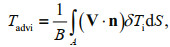 (1)
(1)where i represents each interface, V·n represents the normal velocity at each interface, S is the interfacial area and B is the box volume. δTi is defined as the temperature difference between the interface temperature and the box-averaged mixed layer temperature (MLT, 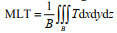
 (2)
(2)where the time tendency of MLT is shown on the left side, and the first five terms on the right-hand side denote advections across the bottom, west, east, south and north ocean interfaces, respectively. Tsurf represents the net surface heat flux. The residual R can contain: horizontal and vertical diffusion, penetrative shortwave radiation through the base of the mixed layer, effects from high-frequency tropical instability waves; computational errors; errors associated with imperfect closure of the temperature budget, including the tendency due to the tendency incurred by the assimilation increment and SST relaxation.
We then break up ocean velocity and MLT into climatological seasonal cycles averaged from 1993 to 2016, and remaining anomalies, to obtain roles of various feedbacks on temperature anomalies. Thus the anomaly of each advection term can be separated into hree parts, i.e., 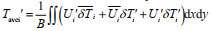
In this manner, Eq.2 can be modified into various terms as,
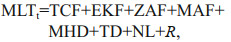 (3)
(3)in which:
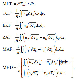

The seven right-hand terms are defined as: thermocline feedback (TCF), Ekman feedback (EKF), zonal advective feedback (ZAF), meridional advective feedback (MAF), mean horizontal dynamical heating term (MHD), thermal damping by the net surface heat flux (TD) and nonlinear advection (NL). As long as we definite the MLT representative of SST, the results are not fundamentally sensitive to varying the mixed layer depth by ±20 m. Other choices of mixed layer depth definition, such as varying with time, which has certain advantages in separating out diabatic and adiabatic vertical processes, however, would make comparison with previous results more difficult and beyond the scope of our study. To obtain both the intraseasonal and interannual variabilities, a Fourier low-pass filter with a cutoff period of 30 days was then applied (Walters and Heston, 1982). More details and discussions of the applied temperature budget method can also be found in Guan and McPhaden (2016).
3 RESULT 3.1 Air-sea anomalies in the equatorial Pacific during 2014–2015Hovmüller diagrams of the basic air-sea anomalies recording the developments of 2014 and 2015 El Niño events are presented in Figs. 1 & 2. In early 2014, two strong WWBs occurred in the western equatorial Pacific, propagating downward Kelvin waves that rapidly spread to the east, as two eastward increases in SSH. Along with the eastward SSH anomalies, negative SSH anomalies soon appeared in the western Pacific, leading to an anomalous SSH zonal gradient across the equatorial Pacific. It could be speculated that this thermocline would have an abnormal tilt, with warm water accumulating from west to east. While the WWBs changed the subsurface ocean, they also drove anomalous eastward ocean surface currents through direct sea surface friction, which propagated to the central-eastern Pacific. Forced by these two processes, SST warmed in the central-eastern Pacific, then with a weak WWB in April, the SST anomaly in the eastern Pacific reached 1℃, suggesting that a strong El Niño event was very likely coming as reported.

|
| Fig.1 Air-sea anomalies in the equatorial Pacific Ocean in 2014 From left to right: NOAA ERDDAP zonal wind stress, AVISO SSH, OSCAR surface zonal current, OISSTv2 SST. Anomalies were obtained by subtracting their corresponding climatology annual means. |

|
| Fig.2 Same as in Fig. 1, but for 2015 |
However, the WWBs did not last, but an abnormal easterly wind occurred in May 2014, and gradually developed into a strong EWB event in June. It piled up the warm water back to the west, and positive SSH anomalies replaced the negative trend in the western Pacific and the eastward current anomalies disappeared in the central-eastern Pacific (Fig. 1). Finally, SST showed negative anomalies in the central-eastern Pacific. Thus, the predicted strong El Niño, in the absence of WWBs and the underlain abnormal eastward current, faded away. However, according to the SSH and SST fields, there were still weak positive abnormal signals across the ocean basin, and although it failed to develop into a super El Niño event, they indicated that the whole equatorial Pacific was full of "energy".
In 2015, WWBs almost ran through the whole year, primarily occurring in the western Pacific and gradually moving eastward to around the dateline after July. A tenable zonal gradient of SSH anomalies could also be found through the year, and a strong abnormal oceanic current pushed the warm water eastward. With the continuous sea-air coupling processes, cooling SST anomalies appeared in the western equatorial Pacific, while the warming SST anomalies intensified in the central-eastern Pacific with a peak of 4℃ in November. An El Niño event then developed as the one of the three strongest recorded, along with those in 1982–1983 and 1997–1998.
Though the intraseasonal wind bursts and induced oceanic processes seemed to play an essential role in the development of the predicted "super" 2014 El Niño and the extreme 2015 El Niño, their quantitative contributions is still not clear, especially on the intraseasonal time scale. Therefore, we conducted a temperature budget analysis to quantify the role of various oceanic feedbacks in the evolution of the 2014–2016 events.
3.2 Temperature budget analysis on 2014–2016 El Niño eventsWe used the ECCO2 product to perform a temperature budget analysis in the ocean mixed layer within the Niño3 and Niño4 key regions. Figure 3 shows the MLT anomalies averaged in each Niño region. The MLT anomalies generally depict well the temperature evolution of 2014–2016 warm events observed from OISSTv2, with differences probably due to averaging in the mixed layer. Positive MLT anomalies were firstly noticed in the Niño4 region in February, and then found in the Niño3 region, which exceeded 0.5℃ at the end of March and peaked in mid-May 2014. In both regions, these warm MLTs began to decrease from June, and even dropped into negative values in the central Pacific, indicating the failure of a super El Niño event (Figs. 1 & 2). However, these warm trends returned after autumn 2014, and continued to grow in 2015 in both regions. The Niño3 MLT anomaly reached its peak of 3.2℃ in December, which was much greater than 1.5℃ in the Niño4 region.

|
| Fig.3 MLT anomalies from ECCO2 (solid line) and SST anomalies (dashed line) from OISSTv2 from January 2014 to January 2016 in the Niño3 and Niño4 regions, respectively Anomalies were obtained by subtracting their corresponding climatology annual cycles. Pink shade indicates key periods of El Niño events, same as in Figs. 4, 5, 6, and 8. |
Before the analysis on various budget terms, we checked the budget conservations for both regions. Both the Niño3 and Niño4 regions have very good conservations, where the sums of the seven air-sea feedback terms closely coincide with the corresponding MLT tendencies (MLTt), with correlation coefficients of 0.93 and 0.92, respectively (Fig. 4).

|
| Fig.4 Heat conservations from Eq.3 for the Niño3 (a) and Niño4 (b) regions Correlation coefficients between MLTt and Fall are presented as r. Fall is the sum of all the feedback terms on the right-hand side of Eq.3 except for R. |
The abnormal changes of temperature budget terms in the Niño3 region from January 2014 to January 2016 are depicted in Fig. 5a. In early spring 2014, the MLT tendency showed an abrupt peak of about 0.8℃/month, leading to a rapid warming with a peak of 1.0℃ in May. Among the positive feedbacks, the EKF led the MLTt contributed the most, with a maximum amplitude of 0.4℃/month. ZAF was the second largest positive feedback terms (reaching approximately 0.25℃/month), followed by TCF (approximately 0.18℃/month), and both the ZAF and TCF lag MLTt. Then in mid-May, MLTt turned negative, so the warm MLT anomaly was weakened to below 0.5℃ in the boreal summer. Within this period, the EKF tended to be a negative effect and still led the variability of negative MLTt. ZAF also changed negative, with its largest contribution in July. Interestingly, TCF maintained a weak positive effect from March to July 2014. The sea surface net heat flux term was the strongest negative feedback term that dampened the temperature anomalies. The MHD and nonlinear terms were generally positive and MAF was very weak. Thus, we conclude that EKF and ZAF are the two dominant oceanic feedbacks in developing the warm event in the spring of 2014 and also its decay in June.

|
| Fig.5 Individual temperature budget terms superimposed on the MLT anomalies in the Niño3 (a) and Niño4 (b) regions |
In September 2014, a weak warming in MLT was found, but all positive feedback terms were small, which did not allow the MLT anomalies to grow further. In 2015, the Niño3 MLTi became positive again in March, and reached its first peak of 0.45℃/month in the middle of April. Among the positive feedbacks, ZAF and TCF were the first two significant contributors, leading to the rapid onset of a warm event with the MLT anomaly reaching above 1.2℃ in June. Moreover, the two positive ZAF and TCF continuously maintained their positive contributions. Two more peaks of MLTi were the found in September and November, of 0.45℃/month and 0.22℃/month, respectively. EKF had two significant jumps, dominating these two MLTi increases. TD and NL were negative feedbacks in the onset of 2015 El Niño event. With the combined contributions of positive ZAF, TCF, and EKF, the warm MLT anomalies rose continuously and peaked as high as 3.0℃, at the end of 2015.
In the Niño3 region, the residual R was mostly negative during 2014–2016, which is relatively small compared to other key terms (i.e., MLTi, TCF, ZAF, and EKF) during the key development or decay periods of the event (i.e., February–June 2014 and February–September 2015). The negative tendency of R may result from some combination of neglected physical processes in our budget formulation and/or from assimilation increments.
Figure 6 shows the variability of different oceanic variables behind the corresponding feedback terms. As we know, ZAF and EKF reflect the mean temperature advection by the anomalous zonal current and vertical current respectively, while TCF reflects the anomalous temperature advection by the mean vertical upwelling at the base of the mixed layer. We looked more detailed into ZAF via the east boundary and west boundary in each Niño region, and found that zonal current anomalies around the west boundary were generally stronger than that in the east boundary. The west-boundary zonal current anomalies showed a significant negative correlation with vertical bottom current anomalies after July 2014, but were insignificant during March–July 2014.

|
| Fig.6 Corresponding oceanic anomalies behind various oceanic feedback terms in Fig. 5 in the Niño3 (a) and Niño4 (b) regions Anomalies of MLT, half of MLT tendency and temperature gradient at the bottom (δTB) refer to the right y-axis, while the anomalies of zonal current at the west boundary (uW) and east boundary (uE), as well as vertical current at the bottom (wB), refer to the left y-axis. |
In early February 2014, an anomalous eastward current appeared around the west boundary of the Niño3 region, advecting warm water to the east. At the same time, anomalous downwelling formed, inhibiting the cold-water transport to the surface and promoting the surface warming. The temperature gradient at the bottom and the zonal current at the eastern boundary showed weak variability in February–March, and thus made a negligible contribution to MLT warming. In mid-march, MLT began to show a warm anomaly, and the vertical temperature gradient at the bottom also began to show a positive anomaly, indicating that the mean upwelling was bringing warmer subsurface water to the surface. However, the anomalous bottom downwelling suddenly turned into an abnormal upwelling at the end of April and began to impede the continued MLT warming. This anomalous upwelling was related to the absence of WWBs and occurrence of an EWB in April (Fig. 2). Then at the end of May, the zonal current anomalies at both the western and eastern boundaries turned westward, beginning to transport warm water to the east and pull the Niño3 MLT anomaly back to normal.
During the development of the extreme 2015 El Niño, zonal current anomalies remained strong and eastward, transporting warm water continuously to the east. The zonal current anomalies at the west boundary were stronger than that at the east boundary, and had two peaks in late April and October. At the bottom, the temperature gradient present positive anomalies and the anomalous vertical upwelling continued through most of the year. These combined oceanic anomalies generated continuous air-sea feedbacks, resulting in the formation of an extreme warm event.
3.2.2 Niño4 regionIn the Niño4 region further west, the MLT tendencies were much weaker. A clear positive MLT tendency was found in January–March of 2014, with a peak of 0.4℃/month in February. In early 2014, NL was found to be the leading positive process driving this warming trend, other than EKF in the Niño3 region. NL was mainly attributed to the nonlinear effect from the bottom interface of the mixed layer (figures not shown), which might be related to the two strong WWBs and tropical cyclones during January–February 2014 (Puy et al., 2016). Hence, the ZAF was a second contributor.
WWBs rapidly drive an abnormal eastward current, up to 0.15 m/s, pushing the warm water of the warm pool to the east and warming the central Pacific through zonal advection (Fig. 6). At the same time, the wind anomaly excited the oceanic anomalous downwelling, but its contribution to the MLT warming (that is EKF) was negligible due to the small mean vertical temperature gradient. Similarly, the TCF is also small since the anomaly of vertical temperature gradient anomalies at the bottom of the mixed layer is small (the red solid line in Fig. 6). The easterly wind anomaly occurs at the end of June 2014, and triggered an anomalous westward current at the eastern boundary of Niño4, producing cold advections that pushed warm water back to the western Pacific, leading to the decline of the 2014 event.
During the evolution of the 2015 El Niño event, ZAF was the leading positive feedback term in the onset phase, mainly induced by the eastward zonal current at the western boundary (Fig. 6). MHD played an important role in the late MLT developing phase after July, comparable to the ZAF (Fig. 5). TCF presented as a stable weak positive feedback and the TD dampened the MLT anomalies. It is noteworthy that NL had a strong damping effect on MLT growth in Niño4, which was even stronger than TD from July to November.
To summarize, in the onset of the 2014 El Niño event, the positive EKF and ZAF, induced by the anomalous vertical downwelling and eastward current, were the two leading contributors. In late April, EKF surprisingly turned into negative by anomalous upwelling, bringing the subsurface cold water into the surface layer and making the surface water cooler. Then, the westward current anomaly induced by EWBs in June further lowered this warming event via negative ZAF. In contrast to 2014, in the developing phase of the 2015 event, positive ZAF induced by the anomalous eastward current was the largest positive term, which continuously warmed the eastern Pacific. Meanwhile, both TCF and EKF were positive feedbacks, accelerating the warm trend.
3.3 Comparison with 1997–1998 El NiñoThe 1997–1998 El Niño event is well-known as a classical extreme El Niño on record. The oceanic and atmospheric changes in the equatorial Pacific during the development of the extreme El Niño in 1997 are depicted in Fig. 7. A series of westerly anomalies were observed in the western Pacific, which drove the oceanic feedbacks continuously throughout the year. By the end of the year, the zonal difference of SSH anomalies had reached more than 70 centimeters, and anomalous eastward zonal currents could be found along the entire equatorial Pacific, making the SST anomaly in the eastern Pacific as high as 4℃.

|
| Fig.7 Same as in Fig.1, but for 1997 |
Both the 1997 and 2014 events, experienced strong WWBs in the early spring, which forced similar SSH anomalous patterns and surface currents warming the central-eastern Pacific. However, the western Pacific in 1997 was characterized by a strong cold SST anomaly, indicating that the heat center of western Pacific warm pool shifted to the east. As speculated in McPhaden (2015), in 2014, the Indo-Pacific convective depression center did not shift eastward in response to WWBs, so that positive Bjerknes feedbacks did not further develop. Therefore, after June, the disappeared westerly winds terminated the 2014 super event, in contrast to the extreme 1997 El Niño that developed when the continuous westerlies became even more powerful and moved further eastward.
As two of the three recorded extreme El Niño events, the 2015 El Niño was similar to the 1997 El Niño but under different air-sea conditions. As shown in Fig. 7, the WWBs in 1997 were more intense than 2015 and had a tendency to move eastward, pushing the warm water rapidly to the east of the dateline. In 1997, the eastward current anomalies occupied the whole basin, while in 2015, the eastward anomalies were concentrated in the western equatorial Pacific. Moreover, SST anomalies in 2015 appeared earlier than in 1997, which were related to the abnormal background field left by the 2014 warm event. These characteristics are consistent with previous studies (e.g., Lim et al., 2017; Xue and Kumar, 2017). Therefore, the strongest warming anomalies were found further east in 1997, which was characterized as a typical eastern Pacific El Niño, while the 2015 event is more like a mixture type of eastern Pacific and central Pacific events (e.g., Paek et al., 2017; Xu et al., 2017).
The various air-sea processes that determined the 1997–1998 El Niño, based on temperature budget analysis are depicted in Fig. 8. In the Niño3 region (Fig. 8a), EKF presented as the largest positive feedback in the early developing phase of the 1997–1998 El Niño with peaks in January, April and June, followed by positive ZAF and TCF. The ZAF and TCF actively increased during the late developing phase of 1997 (during September to December), exceeding 0.5℃/month. TCF became a strong positive feedback term from March 2015, earlier than that in 1997, which is consistent with Zhang and Gao (2017) suggesting the role of positive subsurface thermal anomalies left over from 2014 in leading the 2015 event. In the Niño4 region, the feedback terms were much smaller. ZAF and NL were the main positive processes in early 1997, while in the late developing phase, ZAF and MHD became the leading two positive processes, similar to the 2015 event in the Niño4 region.

|
| Fig.8 Same as in Fig. 5, but for the periods 1997–1999 |
We explored the role of various oceanic feedbacks in the 2014–2016 El Niño events, based on a detailed temperature budget analysis. Using the 3-daily output of an ECCO2 product, we accessed the role of oceanic feedbacks in response to both intraseasonal wind busts and interannual ENSO low frequencies. The analyses were focused in the Niño3 and Niño4 regions to explore the variability across the central and eastern Pacific. In the eastern Pacific, the Ekman feedback dominated the 2014 spring warming, induced by anomalous downwelling forced by a series of westerly wind bursts. Zonal advective feedback followed as a second contributor. These two processes turned sequentially into negative effects on temperature changes in response to easterly wind bursts in May, which dramatically led to a decay in the 2014 El Niño event. In the 2015 extreme El Niño, zonal advective feedback and thermocline feedback were the two leading processes that prompted an early warming in the Niño3 region, while in the late developing stage, two significant jumps dominated the warming tendencies induced by westerly wind anomalies. In the central Pacific Niño4 region, the Ekman feedback and thermocline feedback were largely reduced due to small vertical temperature gradients, so that zonal advective feedback was generally the largest positive oceanic feedback. Besides, nonlinear term also played a role in the 2014 spring warming.
Budget analysis can provide quantitative diagnosis of various oceanic feedback terms contributing to the temperature evolution of ENSO events. Particularly, our budget method allows us to be more focused on the temperature variabilities averaged in the key Niño regions, since the tendency of domain temperature and advections are not affected by the heat redistributed internally by small-scale processes inside the selected regions (Lee et al., 2004), as well as the effects of volume transports whose temperature is the same as the domain average (Zhang and McPhaden, 2010). We note that the ECCO2 reanalysis data used in this study can contain the impacts of assimilation increments, induced when the model output is corrected for the model deficiencies to produce realistic ENSO SSTs. Assimilation increment can compensate for a particular error listed in the following or their combinations: inaccuracy of prescribed surface heat flux, mis-representations of advection and/or mixing due to inaccurate wind forcing, and limitations due to model physics such as mixing parameterizations or diffusion coefficients. To assess where the increments are from for these ECCO2 assimilations at each time step and how they affect oceanic feedbacks in the budget equation are important, however, beyond the scope of this study. We have included it in the residual term and it is found to have no significant impact on our main results.
The present work is focused on the oceanic feedbacks that combined intraseasonal and interannual oceanic processes in modulating the onset of El Niño events, which has advantages over previous studies based on monthly data that might miss the intraseasonal processes (e.g., Ren et al., 2017). For example, we found that Ekman feedback had significant effects on the early onset of El Niño and also the decay of the 2014 event via its jump-like variability on an intraseasonal time scale. The intraseasonal vertical current variability behind Ekman feedback in the central-eastern Pacific is related to remotely forced equatorial Kelvin waves (e.g. Zhang, 2001; Kutsuwada and McPhaden, 2002; McPhaden, 2002; Marshall et al., 2009). The remote effect of intraseasonal variability on the eastern Pacific is via downwelling Kelvin waves generated by westerly wind anomalies in the western Pacific. These Kelvin waves are remotely forced by WWBs in the western Pacific, propagate eastward along the thermocline to the central and eastern Pacific and deepen the thermocline, which also modify the thermal effect of the equatorial upwelling in the eastern Pacific (Zhang, 2001). Considering that the oceanic feedbacks on an intraseasonal time scale are even more complicated and more important in terms of response to wind bursts and excited Kelvin waves, and that more factors such as salinity have recently been found to play important roles on the ENSO events (Zhang et al., 2012; Zheng and Zhang, 2015; Guan et al., 2019b; Zhi et al., 2019), further studies are needed to better understand ENSO dynamics.
5 DATA AVAILABILITY STATEMENTThe OISSTv2 data are available at www.ncdc. noaa.gov, the SSH data are from the AVISO altimeter at www.aviso.altimetry.fr, the wind stress data from NOAA/ERDDAP are at https://coastwatch.pfeg.noaa.gov/erddap, and OSCAR surface ocean current at http://podaac.jpl.nasa.gov. The ECCO2 outputs can be found at ftp://ecco.jpl.nasa.gov/ECCO2.
6 ACKNOWLEDGMENTWe thank Dr. Michael J. McPhaden of NOAA/ Pacific Marine Environmental Laboratory for his valuable comments. We acknowledge NOAA and NASA JPL for their valuable observations and model products.
Bjerknes J. 1969. Atmospheric teleconnections from the equatorial Pacific. Monthly Weather Review, 97(3): 163-172.
DOI:10.1175/1520-0493(1969)097<0163:ATFTEP>2.3.CO;2 |
Cai W J, Borlace S, Lengaigne M, van Rensch P, Collins M, Vecchi G, Timmermann A, Santoso A, McPhaden M J, Wu L X, England M H, Wang G J, Guilyardi E, Jin F F. 2014. Increasing frequency of extreme El Niño events due to greenhouse warming. Nature Climate Change, 4(2): 111-116.
DOI:10.1038/nclimate2100 |
Chen D K, Lian T, Fu C B, Cane M A, Tang Y M, Murtugudde R, Song X S, Wu Q Y, Zhou L. 2015. Strong influence of westerly wind bursts on El Niño diversity. NatureGeoscience, 8(5): 339-345.
DOI:10.1038/ngeo2399 |
Chen L, Li T, Wang B, Wang L. 2017. Formation mechanism for 2015/16 super El Niño. Scientific Report, 7(1): 2 975.
DOI:10.1038/s41598-017-02926-3 |
Dong L, McPhaden M J. 2018. Unusually warm Indian Ocean sea surface temperatures help to arrest development of El Niño in 2014. Science Reports, 8(1): 2 249.
DOI:10.1038/s41598-018-20294-4 |
Ducet N, Le Traon P Y, Reverdin G. 2000. Global highresolution mapping of ocean circulation from TOPEX/Poseidon and ERS-1 and -2. Journal of Geophysical Research:Oceans, 105(C8): 19 477-19 498.
DOI:10.1029/2000JC900063 |
Fedorov A V, Philander S G. 2000. Is El Niño changing?Science, 288(5473): 1 997-2 002, https: //doi.org/10.1126/science.288.5473.1997.
|
Fedorov A V, Philander S G. 2001. A stability analysis of tropical ocean-atmosphere interactions:bridging measurements and theory for El Niño. Journal of Climate, 14(14): 3 086-3 101.
DOI:10.1175/1520-0442(2001)014<3086:ASAOTO>2.0.CO;2 |
Guan C, Hu S J, McPhaden M J, Wang F, Gao S, Hou Y L. 2019a. Dipole structure of mixed layer salinity in response to El Niño-La Niña asymmetry in the tropical Pacific. Geophysical Research Letters, 46(12): 12 165-12 172.
DOI:10.1029/2019GL084817 |
Guan C, McPhaden M J, Wang F, Hu S J. 2019b. Quantifying the role of oceanic feedbacks on ENSO asymmetry. Geophysical Research Letters, 46(4): 2 140-2 148.
DOI:10.1029/2018GL081332 |
Guan C, McPhaden M J. 2016. Ocean processes affecting the twenty-first-century shift in ENSO SST variability. Journal of Climate, 29(19): 6 861-6 879.
DOI:10.1175/JCLI-D-15-0870.1 |
Halkides D J, Lucas L E, Waliser D E, Lee T, Murtugudde R. 2011. Mechanisms controlling mixed-layer temperature variability in the eastern tropical Pacific on the intraseasonal timescale. Geophysical Research Letters, 38(17): L17602.
DOI:10.1029/2011GL048545 |
Halpern D, Menemenlis D, Wang X. 2015. Impact of data assimilation on ECCO2 equatorial undercurrent and North equatorial countercurrent in the Pacific Ocean. Journal of Atmospheric & Oceanic Technology, 32(1): 131-143.
DOI:10.1175/JTECH-D-14-00025.1 |
Harrison D E, Vecchi G A. 1997. Westerly wind events in the Tropical Pacific, 1986-95. Journal of Climate, 10(12): 3 131-3 156.
DOI:10.1175/1520-0442(1997)010<3131:WWEITT>2.0.CO;2 |
Hu D X, Wu L X, Cai W J, Gupta A S, Ganachaud A, Qiu B, Gordon A L, Lin X P, Chen Z H, Hu S J, Wang G J, Wang Q Y, Sprintall J, Qu T D, Kashino Y, Wang F, Kessler W S. 2015. Pacific western boundary currents and their roles in climate. Nature, 522(7556): 299-308.
DOI:10.1038/nature14504 |
Hu S J, Hu D X, Guan C, Xing N, Li J P, Feng J Q. 2017. Variability of the western Pacific warm pool structure associated with El Niño. Climate Dynamics, 49(7-8): 2 431-2 449.
DOI:10.1007/s00382-016-3459-y |
Hu S N, Fedorov A V. 2016. Exceptionally strong easterly wind burst stalling El Niño of 2014. Proceedings of the National Academy of Sciences of the United States of America, 113(8): 2 005-2 010.
DOI:10.1073/pnas.1514182113 |
Hu S N, Fedorov A V. 2019. The extreme El Niño of 2015-2016:the role of westerly and easterly wind bursts, and preconditioning by the failed 2014 event. Climate Dynamics, 52(12): 7 339-7 357.
DOI:10.1007/s00382-017-3531-2 |
Imada Y, Tatebe H, Watanabe M, Ishii M, Kimoto M. 2016. South Pacific influence on the termination of El Niño in 2014. Scientific Report, 6(1): 30 341.
DOI:10.1038/srep30341 |
Ineson S, Balmaseda M A, Davey M K, Decremer D, Dunstone N J, Gordon M, Ren H L, Scaife A A, Weisheimer A. 2018. Predicting El Niño in 2014 and 2015. Scientific Reports, 8(1): 10 733.
DOI:10.1038/s41598-018-29130-1 |
Jin F F, Kug J S, An S I, Kang I S. 2003. A near-annual coupled ocean-atmosphere mode in the equatorial Pacific ocean. Geophysical Research Letters, 30(2): 1 080.
DOI:10.1029/2002GL015983 |
Jin F F. 1997. An equatorial ocean recharge paradigm for ENSO. Part Ⅰ:Conceptual model. Journal of the Atmospheric Sciences, 54(7): 811-829.
DOI:10.1175/1520-0469(1997)054<0811:AEORPF>2.0.CO;2 |
Kutsuwada K, McPhaden M J. 2002. Intraseasonal variations in the upper equatorial Pacific Ocean prior to and during the 1997-98 El Niño. Journal of Physical Oceanography, 32(4): 1 133-1 149.
DOI:10.1175/1520-0485(2002)032<1133:IVITUE>2.0.CO;2 |
Lagerloef G S E, Mitchum G T, Lukas R B, Niiler P P. 1999. Tropical Pacific near-surface currents estimated from altimeter, wind, and drifter data. Journal of Geophysical Research:Oceans, 104(C10): 23 313-23 326.
DOI:10.1029/1999JC900197 |
Lee T, Fukumori I, Tang B Y. 2004. Temperature advection:internal versus external processes. Journal of Physical Oceanography, 34(8): 1 936-1 944.
DOI:10.1175/1520-0485(2004)034<1936:TAIVEP>2.0.CO;2 |
Levine A F Z, McPhaden M J. 2016. How the July 2014 easterly wind burst gave the 2015-2016 El Niño a head start. Geophysical Research Letters, 43(12): 6 503-6 510.
DOI:10.1002/2016GL069204 |
Lian T, Chen D K, Tang Y M, Wu Q Y. 2014. Effects of westerly wind bursts on El Niño:a new perspective. Geophysical Research Letters, 41(10): 3 522-3 527.
DOI:10.1002/2014GL059989 |
Lim Y K, Kovach R M, Pawson S. Vernieres G. 2017. The 2015/16 El Niño event in context of the MERRA-2 reanalysis:a comparison of the tropical Pacific with 1982/83 and 1997/98. Journal of Climate, 30(13): 4 819-4 842.
DOI:10.1175/JCLI-D-16-0800.1 |
Maeda S, Urabe Y, Takemura K, Yasuda T, Tanimoto Y. 2016. Active role of the ITCZ and WES feedback in hampering the growth of the expected full-fledged El Niño in 2014. SOLA, 12: 17-21.
DOI:10.2151/sola.2016-004 |
Marshall A G, Alves O, Hendon H H. 2009. A coupled GCM analysis of MJO activity at the onset of El Niño. Journal of the Atmospheric Sciences, 66(4): 966-983.
DOI:10.1175/2008JAS2855.1 |
McPhaden M J, Zebiak S E, Glantz M H. 2006. ENSO as an integrating concept in Earth science. Science, 314(5806): 1 740-1 745.
DOI:10.1126/science.1132588 |
McPhaden M J. 1999. Genesis and evolution of the 1997-98 El Niño. Science, 283(5404): 950-954.
DOI:10.1126/science.283.5404.950 |
McPhaden M J. 2002. Mixed layer temperature balance on intraseasonal timescales in the Equatorial Pacific Ocean. Journal of Climate, 15(18): 2 632-2 647.
DOI:10.1175/1520-0442(2002)015<2632:MLTBOI>2.0.CO;2 |
McPhaden M J. 2015. Playing hide and seek with El Niño. Nature Climate Change, 5(9): 791-795.
DOI:10.1038/nclimate2775 |
Meinen C S, McPhaden M J. 2000. Observations of warm water volume changes in the equatorial Pacific and their relationship to El Niño and La Nina. Journal of Climate, 13(20): 3 551-3 559.
DOI:10.1175/1520-0442(2000)013<3551:OOWWVC>2.0.CO;2 |
Menemenlis D, Fukumori I, Lee T. 2005. Using Green's functions to calibrate an ocean general circulation model. Monthly Weather Review, 133(5): 1 224-1 240.
DOI:10.1175/MWR2912.1 |
Menkes C E, Lengaigne M, Vialard J, Puy M, Marchesiello P, Cravatte S, Cambon G. 2014. About the role of Westerly Wind Events in the possible development of an El Niño in 2014. Geophysical Research Letters, 41(18): 6 476-6 483.
DOI:10.1002/2014GL061186 |
Min Q Y, Su J Z, Zhang R H, Rong X Y. 2015. What hindered the El Niño pattern in 2014?. Geophysical Research Letters, 42(16): 6 762-6 770.
DOI:10.1002/2015GL064899 |
Moore A M, Kleeman R. 1999. Stochastic forcing of ENSO by the intraseasonal oscillation. Journal of Climate, 12(5): 1 199-1 220.
DOI:10.1175/1520-0442(1999)012<1199:SFOEBT>2.0.CO;2 |
Paek H, Yu J Y, Qian C C. 2017. Why were the 2015/2016 and 1997/1998 extreme El Niños different?. Geophysical Research Letters, 44(4): 1 848-1 856.
DOI:10.1002/2016GL071515 |
Pandey V K, Singh S K. 2010. Comparison of ECCO2 and NCEP reanalysis using TRITON and RAMA data at the Indian Ocean Mooring Buoy point. e-Journal of Earth Science India, 3: 226-241.
|
Puy M, Vialard J, Lengaigne M, Guilyardi E. 2016. Modulation of equatorial Pacific westerly/easterly wind events by the Madden-Julian oscillation and convectively-coupled Rossby waves. Climate Dynamics, 46(7-8): 2 155-2 178.
DOI:10.1007/s00382-015-2695-x |
Reynolds R W, Smith T M, Liu C, Chelton D B, Casey K S, Schlax M G. 2007. Daily high-resolution blended analyses for sea surface temperature. Journal of Climate, 20: 5 473-5 496.
DOI:10.1175/2007JCLI1824.1 |
Ren H L, Wang R, Zhai P M, Ding Y H, Lu B. 2017. Upper-ocean dynamical features and prediction of the super El Niño in 2015/16:a comparison with the cases in 1982/83 and 1997/98. Journal of Meteorological Research, 31(2): 278-294.
DOI:10.1007/s13351-017-6194-3 |
Santoso A, McPhaden M J, Cai W J. 2017. The defining characteristics of ENSO extremes and the strong 2015/2016 El Niño. Reviews of Geophysics, 55(4): 1 079-1 129.
DOI:10.1002/2017RG000560 |
Santoso A, McPhaden M J, Cai W J. 2017. The defining characteristics of ENSO extremes and the strong 2015/2016 El Niño. Reviews of Geophysics, 55(4): 1 079-1 129.
DOI:10.1002/2017RG000560 |
Seiki A, Takayabu Y N. 2007a. Westerly wind bursts and their relationship with intraseasonal variations and ENSO. Part Ⅰ:statistics. Monthly Weather Review, 135(10): 3 346-3 361.
DOI:10.1175/MWR3503.1 |
Seiki A, Takayabu Y N. 2007b. Westerly wind bursts and their relationship with intraseasonal variations and ENSO. Part Ⅱ:energetics over the Western and Central Pacific. Monthly Weather Review, 135: 3 346-3 361.
DOI:10.1175/MWR3503.1 |
Smith S D. 1988. Coefficients for sea surface wind stress, heat flux, and wind profiles as a function of wind speed and temperature. Journal of Geophysical Research:Oceans, 93(C12): 15 467-15 472.
DOI:10.1029/JC093iC12p15467 |
Timmermann A, An S I, Kug J S, et al. 2018. El Niño-Southern Oscillation complexity. Nature, 559(7715): 535-545.
DOI:10.1038/s41586-018-0252-6 |
Walters R A, Heston C. 1982. Removing tidal-period variations from time-series data using low-pass digital filters. Journal of Physical Oceanography, 12(1): 112-115.
DOI:10.1175/1520-0485(1982)012<0112:RTPVFT>2.0.CO;2 |
Wang G M, Hendon H H. 2017. Why 2015 was a strong El Niño and 2014 was not. Geophysical Research Letters, 44(16): 8 567-8 575.
DOI:10.1002/2017GL074244 |
Wu Y K, Chen L, Hong C C, Li T, Chen C T, Wang L. 2018. Role of the meridional dipole of SSTA and associated cross-equatorial flow in the tropical eastern Pacific in terminating the 2014 El Niño development. Climate Dynamics, 50(5-6): 1 625-1 638.
DOI:10.1007/s00382-017-3710-1 |
Wyrtki K. 1975. El Niño-the dynamic response of the Equatorial Pacific Oceanto atmospheric forcing. Journal of Physical Oceanography, 5(4): 572-584.
DOI:10.1175/1520-0485(1975)005<0572:ENTDRO>2.0.CO;2 |
Xu K, Huang R X, Wang W Q, Zhu C W, Lu R Y. 2017. Thermocline fluctuations in the Equatorial Pacific Related to the two types of El Niño events. Journal of Climate, 30(17): 6 611-6 627.
DOI:10.1175/JCLI-D-16-0291.1 |
Xue Y, Kumar A. 2017. Evolution of the 2015/16 El Niño and historical perspective since 1979. Science China Earth Sciences, 60(9): 1 572-1 588.
DOI:10.1007/s11430-016-0106-9 |
Zhai P M, Yu R, Guo Y J, Li Q X, Ren X J, Wang Y Q, Xu W H, Liu Y J, Ding Y H. 2016. The strong El Niño of 2015/16 and its dominant impacts on global and China's climate. Journal of Meteorological Research, 30(3): 283-297.
DOI:10.1007/s13351-016-6101-3 |
Zhang C D. 2001. Intraseasonal perturbations in sea surface temperatures of the equatorial eastern Pacific and their association with the Madden-Julian oscillation. Journal of Climate, 14(6): 1 309-1 322.
DOI:10.1175/1520-0442(2001)014<1309:IPISST>2.0.CO;2 |
Zhang R H, Gao C. 2016. The IOCAS intermediate coupled model (IOCAS ICM) and its real-time predictions of the 2015-2016 El Niño event. Science Bulletin, 61(13): 1 061-1 070.
DOI:10.1007/s11434-016-1064-4 |
Zhang R H, Gao C. 2017. Processes involved in the secondyear warming of the 2015 El Niño event as derived from an intermediate ocean model. Science China Earth Sciences, 60(9): 1 601-1 613.
DOI:10.1007/s11430-016-0201-9 |
Zhang R H, Zheng F, Zhu J S, Pei Y H, Zheng Q N, Wang Z G. 2012. Modulation of El Niño-southern oscillation by freshwater flux and salinity variability in the Tropical Pacific. Advances in Atmospheric Sciences, 29(4): 647-660.
DOI:10.1007/s00376-012-1235-4 |
Zhang R H, Zheng F, Zhu J, Wang Z G. 2013. A successful real-time forecast of the 2010-11 La Niña event. Scientific Reports, 3: 1108.
DOI:10.1038/srep01108 |
Zhang X B, McPhaden M J. 2010. Surface layer heat balance in the Eastern Equatorial Pacific Ocean on interannual time scales:influence of local versus remote wind forcing. Journal of Climate, 23(16): 4 375-4 394.
DOI:10.1175/2010JCLI3469.1 |
Zheng F, Zhang R H. 2015. Interannually varying salinity effects on ENSO in the tropical Pacific:a diagnostic analysis from Argo. Ocean Dynamics, 65(5): 691-705.
DOI:10.1007/s10236-015-0829-7 |
Zheng F, Zhu J. 2010. Coupled assimilation for an intermediated coupled ENSO prediction model. Ocean Dynamics, 60(5): 1 061-1 073.
DOI:10.1007/s10236-010-0307-1 |
Zheng F, Zhu J. 2016. Improved ensemble-mean forecasting of ENSO events by a zero-mean stochastic error model of an intermediate coupled model. Climate Dynamics, 47(12): 3 901-3 915.
DOI:10.1007/s00382-016-3048-0 |
Zhi H, Zhang R H, Lin P F, Shi S W. 2019. Effects of salinity variability on recent El Niño events. Atmosphere, 10(8): 475.
DOI:10.3390/atmos10080475 |
Zhong W X, Cai W J, Zheng X T, Yang S. 2019. Unusual anomaly pattern of the 2015/2016 extreme El Niño induced by the 2014 warm condition. Geophysical Research Letters, 46(24): 14 772-14 781.
DOI:10.1029/2019GL085681 |
Zhu J S, Kumar A, Huang B H, Balmaseda M A, Hu Z Z, Marx L, Kinter III J L. 2016. The role of off-equatorial surface temperature anomalies in the 2014 El Niño prediction. Scientific Report, 6: 19 677.
DOI:10.1038/srep19677 |