1 INTRODUCTION

The higher resolution of the merged dataset reveals that more than 50% of the variability over much of the World Ocean is accounted for by eddies with amplitudes of 5–25 cm and diameters of 100–200 km (Chelton et al., 2007). Mesoscale eddies can be simply classified into two distinct categories depending on their vertical position (surface or subsurface). There is evidence that surface-intensified eddies, as a ubiquitous phenomenon in the ocean, play an essential role in transferring physical, biological, and chemical properties across large spatial and temporal scales (Shapiro and Meschanov, 1991; Chaigneau et al., 2011; Chelton et al., 2011; Gaube et al., 2013; Zhang et al., 2014; Thomsen et al., 2016). Using satellite data and Argo floats, the characteristics and generation mechanisms of surface-intensified eddies in northwestern tropical oceans have been well studied (Kashino et al., 2013; Chen et al., 2015b). Another type of eddy that is largely invisible at the sea surface is known as a subsurface-intensified eddy (SSE). SSEs typically have their core in a subsurface layer and exhibits, by nature, a completely distinct vertical structure from surface-intensified eddies. SSEs are characterized by oceanographic anomalies indicative of foreign water of distant origin. Isopleths of subsurface anticyclonic (cyclonic) eddies tend to dome (bowl) in shallow water depths and bowl (dome) in deeper water (McGillicuddy, 2015).

Unlike surface eddies, which can be characterized from satellite data, the discovery of SSEs is primarily through hydrographic data. Despite these difficulties in observation, SSEs have been found in many parts of the global ocean, such as Mediterranean water eddies (Meddies) in the North Atlantic Ocean (IsernFontanet et al., 2004; Filyushkin et al., 2014; Damien et al., 2017; Radko and Sisti, 2017), Red Sea outflow water eddies (Reddies) in the Indian Ocean (Shapiro and Meschanov, 1991), California undercurrent eddies (Cuddies) in the eastern North Pacific Ocean (Collins et al., 2013; Pelland et al., 2013), 13℃ eddies in the eastern South Pacific Ocean (Johnson and McTaggart, 2010; Combes et al., 2015). SSEs were also observed in the Arctic Ocean (Brannigan et al., 2017), the Bay of Bengal (Gordon et al., 2017) and in Drake Passage (Brearley at al., 2014).

The northwestern tropical Pacific is characterized by a complicated ocean circulation structure. The North Equatorial Current (NEC) bifurcates into the northward-flowing Kuroshio and southward-flowing Mindanao currents (MC) as it approaches the coast of the Philippines (Qu et al., 2012; Schonau et al., 2015). MC carries the north Pacific tropical water and the north Pacific intermediate water. The main body of the NEC is confined to water shallower than 500 m. The MC veers eastward at the southern tip of Mindanao Island near 5°N to form the North Equatorial Countercurrent (NECC) (Qiu et al., 2015). Below the surface currents, the Luzon Undercurrent (LUC) that flows equatorward beneath the Kuroshio Current, the poleward-flowing Mindanao Undercurrent (MUC) beneath the MC and eastwardflowing North Equatorial Undercurrent (NEUC) below the NEC form a highly variable subsurface current system (Qu et al., 1997; Qu and Lukas, 2003). Besides, the northwestern tropical Pacific is a region where interhemispheric waters converge. To clarify the vertical structures of the currents, we plot in Fig. 1a the latitude-depth sections of zonal geostrophic velocity U(y, z) along 140°E based on cruise observations conducted by R/V Kexue in April 2017. A Sea-Bird SBE 911 conductivity-temperature-depth (CTD) with dual temperature and conductivity sensors was used to measure the conductivity and temperature profiles at 24 Hz. The accuracy of conductivity was 0.0003 S/m, and the temperature was 0.001℃ for CTD. The horizontal geostrophic velocities can be derived as the following:

where Δϕ is dynamic height that can be calculated from temperature and salinity, A and B denote CTD stations, L is the distance between the stations, g is gravitational acceleration, and f is the Coriolis parameter.

Recently, mooring observations showed that SSEs also occasionally observed in the northwestern tropical Pacific Ocean. At least two groups of SSEs near the Philippines coast were detected: one originating from the southeast and the other from the east (Chiang et al., 2015). Using a subsurface mooring (4°N, 143°E), Zhang et al. (2017) reported a subthermocline eddy that enhanced shear instability. An extra-large subsurface anticyclonic eddy (horizontal scale of 470 km) was detected east of Taiwan, China, and was found to carry Subtropical Mode Water westward over 1 500 km (Nan et al., 2017). A deep baroclinic eddy induced by a surface cyclonic eddy is detected in the northwestern South China Sea (Chen et al., 2015a). Later, utilizing model data, SSE characteristics in the northwestern Pacific Ocean, such as distribution, size, amplitude, polarity and longevity, have been reported and the results show SSEs are strongly nonlinear during most of their lifetime, which implies that they can trap interior fluid during translation (Xu et al., 2019).

However, compared with surface-intensified eddies, our understanding of SSEs in the northwestern Pacific Ocean remains observationally fragmentary and theoretically defective due to spatial and temporal limitations of in situ subsurface observations. Although the main horizontal distributions and kinematic properties of SSEs have been investigated during the last decade, very little is known about their vertical structure, their impact on heat transport, and their generation mechanisms. The rest of this paper is structured as follows. Section 2 describes the data and methodology used. In Section 3, we analyze the characteristics of the vertical structures of the SSE (Section 3.1), heat transport induced by SSE (Section 3.2) and energy source of SSE (Section 3.3). The paper ends with a summary of the results (Section 4).

2 DATA AND METHOD 2.1 Model description

The Oceanic General Circulation Model for the Earth Simulator (OFES) was used in this study. It is based on the Modular Ocean Model V.3 with a spherical grid in the horizontal and z-coordinates in the vertical. Its domain extends from 75°S to 75°N, excluding the Arctic region, with 0.1° horizontal grid spacing. The vertical spacing varies from 5 m at the surface to 330 m near the bottom. After a 50-year climatological spin-up, the model was forced by daily surface wind stress, heat flux and salinity flux based on National Centers for Environmental Prediction reanalysis products. The readers are referred to Masumoto et al. (2004) and Sasaki et al. (2008) for more details about the configuration and evaluation of this model. The OFES products have been extensively analyzed by a number of early studies and the results have demonstrated the promising capability of the model in representing realistic variability of different spatial and temporal scales in the ocean (Dutrieux, 2009; Qu et al., 2012; Kashino et al., 2013; Qiu et al., 2015). The validation of the model data and the eddy identification procedure used in this paper can be found in Xu et al. (2019). Comparison of model data and altimeter observations indicated that the model data and our detection algorithm could satisfactorily reproduce eddy activities.

2.2 Subsurface eddy identification

Our detection method is based on Okubo-Weiss parameter contours (Isern-Fontanet et al., 2006). The Okubo-Weiss parameter (W) is defined as:

where and are the normal and shear components of strain, respectively, and is the relative vorticity. The contour search in this study was performed using a specified threshold value (W₀=-0.2σ_w). Here, σ_w, which represents the standard deviation of the W field, was calculated at each time step for the selected domain and depth. The W field was first smoothed with halfpower filter cutoffs of 1.5°×1.5° to reduce the W noise. The shape error was defined as the ratio between the sums of the total area of deviations from the circle to the area of the circle (Kurian et al., 2011). It was calculated for each closed contour; those closed contours with a shape error of < 70% were defined as eddies. The center location of each identified eddy was defined as the centroid of the outermost closed contour of W₀. Finally, only the area of W₀ contours larger than 50 km×50 km are considered as eddies. Because eddies have a deep vertical structure, a deep surface eddy can have signatures at deeper depths (>400 m), and conversely a few SSEs can have weak signatures at the surface. To avoid double counting, only those eddies with their entire body deeper than 45 m were counted as SSEs (i.e. those that could not be detected in the upper eight layers of the model data).

3 RESULT 3.1 Composite structure of subsurface eddies

Figure 1c & d shows the spatial occurrence and dominance of subsurface anticyclonic eddies (SSAEs) and subsurface cyclonic eddies (SSCEs). Here, eddy frequency was defined as the percentage of time that a point was located within a cyclonic or anticyclonic eddy. For example, eddy frequency at a specific location was considered about 10% if occupied by eddies for 10 out of 100 days. In our study region, SSEs were mainly distributed between 9°N and 17°N in open ocean and east of the Philippines coast (Fig. 1c & d). In addition, SSAEs were observed more frequently than SSCEs to the east of the Philippines, which is consistent with previous observational studies (Combes et al., 2015; Song et al., 2017).

To delineate the vertical structure of SSEs, we generated composite maps of eddy anomalies for all detected SSEs. The eddy-induced anomaly for a field at a given time and depth in the analysis was calculated by subtracting the horizontal average of the field over a box field of 5°×5° bin, centered around the eddy. The anomalies are in the depth surface. All identified SSEs were selected for the reconstruction by averaging the snapshots, regardless of their lifespan. Figure 2 shows the vertical section of the composite SSE along the zonal direction at Δy=0. The positive temperature anomaly core of SSAEs was located at around 650 m, deeper than the SSCE negative core, which was found at 500 m (Fig. 2a & b). Temperature anomalies greater than 0.3℃ extended from 600 m to 800 m for SSAEs and 400 m to 800 m for SSCEs. Interestingly for SSAEs was the occurrence of a clear, near zero temperature anomaly that coincided with maximum velocity at 400-m water depth. The water in a SSAE was colder than surrounding water above 400 m and warmer below 400 m. Negative temperature anomalies prevailed throughout a SSCE. Both SSAEs and SSCEs showed two salinity anomaly cores of different polarities (Fig. 2c & d). SSAEs displayed positive anomalies in their cores and negative anomalies below their cores. The opposite was true for SSCEs; they exhibited negative and positive anomalies in and below their cores, respectively.

The mean vertical structures of meridional velocity associated with SSAEs and SSCEs along the zonal section at Δy=0 are shown in Fig. 2e & f. As expected, maximum speeds prevailed in subsurface layers. In the subsurface, the meridional velocity varied from a few cm/s near the center to 10–13 cm/s approximately halfway between the composite eddy center and its edge. The maxima velocity in the very surface maybe the result of surface eddies which is right above the subsurface eddies. Note that the SSAE and SSCE surveyed by Nan et al. (2017) in east of the Philippines had a maximum swirl speed of 0.4 m/s at ~400 m depth and were located between 200 m and 800 m. In agreement with Nan et al. (2017), the SSE identification method used here revealed that both SSAEs and SSCEs have an obvious maximum velocity at ~400 m depth along the zonal section at Δy=0. These vertical velocity structures give us confidence in our identification method.

The potential vorticity (PV) and PV anomaly (PVA) are particularly suited to identify and describe SSEs (Thomas, 2008; Zhang et al., 2017). The PV is defined as:

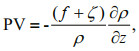
where is the vertical component of the is the vertical component of the relative vorticity, f is the Coriolis parameter, and ρ is the potential density. Analysis of the PVA structure crossing the SSAE center (Fig. 3a) showed that the combination of the intense anticyclonic vorticity and the negative stratification anomaly yields an anomalously low PV between 200 m and 800 m. The largest PVA within an SSAE reached -1.5×10^-11/(m·s), and resided in the eddy center where stratification is weakest. In contrast, SSCEs were characterized by obvious positive PVA from 50 m to 400 m (Fig. 3b). This is the result of near-surface isopycnals deflecting downward by convergence at the SSCE center. Figure 4 shows the vertical section of normalized relative vorticity (ζ/f) of the composite SSAE and SSCE. It is clear that PV is largely dominated by planetary PV.

3.2 Heat transport of subsurface eddies

Theoretical and observational analyses indicated that mesoscale eddies can transport heat, salt and sea water constituents through individual movements (Volkov et al., 2008; Dong et al., 2014; Zhang et al., 2014). The amount of water trapped inside an eddy depends on the ratio of its average rotational speed to its translation speed, also known as the nonlinearity parameter. An eddy is nonlinear when this ratio exceeds one and maintains a coherent structure as it propagates (Chelton et al., 2007, 2011). Accordingly, we analyzed the nonlinearity of SSEs in the northwestern Pacific Ocean. The modeling results showed that most of the observed SSEs were nonlinear and about 89% (37%) of tracked SSEs were nonlinear for at least half (all) of their lifetime (Xu et al., 2019). The composite vertical SSE structure (see Section 3.1) implied strong and complex temperature anomalies. This type of anomaly tends to move with a SSE owing to the trapping of water parcels caused by nonlinearity.

We estimated heat transport induced by SSE movement. For a single SSE, the heat anomaly (Q) was calculated as:

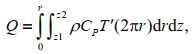
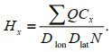
where ρ is the density, C_p is the heat capacity (4 200 J/(kg∙℃)), T′ is temperature anomaly, r is the eddy radius within a specific layer and z is depth layer thickness within a SSE. The vertical integral was calculated by discrete summation over the interpolated vertical levels. In a SSE, Q is dominated by the deeper anomalies that generally span a larger depth range than the shallower anomalies. We set up an average bin with 2.5° meridional width (D_lat) and 2.5° zonal length (D_lon) around each grid point. The heat transport carried by every eddy identified in the OFES was Q·C_x where C_x is the zonal propagation speed of individual eddies. We accumulated the total SSEinduced transport within each bin for whole periods from 2003 to 2013 and divided it by D_lon, D_lat, and the number of snapshots (N). The average eddy-induced zonal heat transport (unit: W/m) is

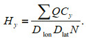
Similar to H_x, we also computed SSE-induced meridional transport

This method is similar to the one used by Zhang et al. (2014) to study eddy-induced mass transport. However, we replaced trapped volume with heat anomalies in their equations to calculate heat transport.

Figures 5 and 6 show the distribution of heat transport by SSAEs and SSCEs in our study region. The heat transport patterns were closely associated with eddy distribution and movement. The heat transport was large between 9°N–17°N where SSEs occur frequently. The distribution of meridional heat transport was on the order of 10³W/m, which is much smaller than the zonal heat transport (10⁴ W/m). This is because of differences in propagation characteristics. Xu et al. (2019) reported that most SSEs move westward with slight equatorward or poleward deflections, and about 10% and 6% of SSAEs and SSCEs, respectively, propagated purely zonally (±1°). The mean zonal velocity from a SSE was about 6.6 cm/s, while it was only about 0.3 cm/s in the meridional direction. In the zonal direction, both SSAEs and SSCEs had negative zonal velocity (westward propagation). With differing thermocline displacement tendencies, the meridional integrated zonal heat transport by SSAEs and SSCEs tended to offset each other to some extent. Hence, the total zonal SSE transport was generally smaller than by either type of SSE alone (Fig. 7a). However, the zonally integrated meridional heat transport of SSAEs and SSCEs combined to give larger values than from either type alone (between 8°N–22°N) (Fig. 7b). The total meridional heat transport peaked at 5°N (~6×10⁹ W) and 20°N (~8×10⁹ W).

3.3 Energy source

The energy in the global ocean is mainly contained as mean kinetic energy (MKE), eddy kinetic energy (EKE), mean available potential energy (MPE) and eddy available potential energy (EPE) (von Storch et al., 2012). An EKE source comprises baroclinic instability (BC) (MPE→EPE→EKE) in which the generation of EKE occurs at the expense of EPE and barotropic instability (BT) (MKE→EKE) that occurs at the expense of MKE. To determine why SSEs frequently occur between 9°N and 17°N and east of the Philippines, and to understand the mechanism of SSE generation in the northwestern tropical Pacific Ocean, we estimated the energy conversion between various components of the total energy. EKE and MKE, the kinetic energies of time-averaged and timevarying circulation, are well defined and can be accurately estimated. However, MPE and EPE, the available potential energies of time-averaged and time-varying circulation, cannot be calculated exactly because they are dependent of the choice of the reference density. Despite these limitations, we can examine the energy transfer rate among different reservoirs.

Given that intrinsic instability processes of ocean currents lead to eddy generation, we first calculated the BT and BC conversion terms following (Oey, 2008).

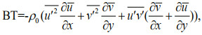
and

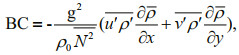
where N² is the square buoyancy frequency, x and y are the longitudinal and latitudinal coordinates, respectively, g is the gravitational acceleration and ρ₀ is the reference density 1 025 kg/m³. Additionally, the prime symbol denotes the deviation from the mean value and the overbar denotes time averaging over 60 days. Here 60-days are sufficiently long to cover the expected periods of instability growths, yet not so long that slow variations of the flow fields will be lumped as "instability". To estimate the deviation squares, we used:

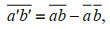
where a is one of the three components of the velocity (u, v, w) and b is a tracer, ab represents the mean flux of b in the direction of a. It is important to note that all of the calculated samples must be averaged over at least several eddy periods to determine sites of persistent instability. In this study, Y=3 years of ensemble-averaged results around 2006 and 2008 were chosen to show the instability patterns and the results were insensitive when Y changed from 2 to 10 years.

Figure 8 shows the energy conversion from MKE to EKE associated with BT. A positive BT indicates that horizontal eddy flux follows the mean momentum gradient where MKE is converted to EKE. A negative BT represents eddy decay that accelerates mean flow where EKE is converted to MKE. The maximal values of BT were south of 7°N and east of the Philippines in the surface layer, which is due to the high horizontal shear energy of western boundary currents. In the subsurface, BT was characterized by unique boundary intensification behavior.

The transfer of MPE to EPE through baroclinic instabilities of mean flow is represented by the abbreviation BC (Fig. 9). A positive BC indicates horizontal eddy density flux against the direction of the mean density gradient where MPE→EPE. Conversely, a negative BC indicates down gradient flux where EPE→MPE. The largest conversion from MPE to EPE occurred in the upper ocean (Fig. 9a). The widespread positive BC values at 20 m are consistent with the energy flow path of EPE along major boundary currents and frontal zones. In the subsurface layers, the most noticeable feature of BC was the prevailing positive value between 9°N and 17°N (Fig. 9).

There is an exchange that represents the conversion between MPE and EKE, which is defined as: , here PKC is the conversion term between eddy potential energy (EPE) to eddy kinetic energy (EKE). It measures the strength of baroclinic production and is a significant source of EKE. It is associated with dense fluid sinking and buoyant fluid rising as part of baroclinic instability. A positive PKC drains energy from EPE to EKE, and vice versa for a negative PKC (Oey, 2008; Yang et al., 2013; Magalhães et al., 2017). The horizontal PKC pattern showed similarities to BC in subsurface layers (Fig. 10). For example, a positive PKC was mainly located between 10°N and 15°N. North and south of this region were negative, indicating that EKE was transferred back to the mean flow. Comparing the pattern of the two baroclinic conversion terms (MPE to EPE and EPE to EKE) with the spatial distribution of SSE occurrence (Figs. 9, 10 & 1), good agreement was found, which suggests that the conversion for both MPE→EPE and EPE→EKE contributed to the increase of EKE in the subsurface.

As shown in a depth section at 143°E, the highest values exceeded 2×10^-5 W/m³ and 1.3×10^-4 W/m³ for BC and PKC, respectively. Positive BC and PKC values were located roughly at 9°N–17°N and 9°N–15°N, respectively, and trend to the north with increasing depth (Fig. 11). Negative conversion values were below the positive patches and the interface between them deepens northward from 200 m at 9°N to 600 m at 15°N. These depths cover the interface between the surface westward-flowing NEC and subsurface eastward-flowing NEUC. The northward shift is associated with meridional movement of NEC bifurcation, which is depth dependent. On average annually, the shift occurs from about 13.3°N near the surface to north of 20°N at depths around 1 000 m (Qu and Lukas, 2003). Note that when the NEC moves north or south, there can be accompanied meridional movement of the NEC and NEUC interface. Thus, meridional movement of the NEC/NEUC can contribute to SSE generation in the study region. To estimate the robustness of our results and study possible SSE energy sources, the vertical profile of mean energy conversion was calculated for the area east of the Philippines coast (region 1: 0°–22°N, 120°E–140°E) and in latitude bands between 9°N–17°N east of 140°E (region 2), where SSEs are frequently observed.

In region 1, all of the energy conversions showed maximum values in the surface. The BT was dominant in the upper 300 m because of the strong horizontal shear energy from the NECC. With increases in depth, BT decreased drastically. However, it remained an important source of subsurface EKE below 600 m, where it was the largest of the three conversion parameters. The mean PKC reached its maximum value at ~400 m and changed around 600 m with positive values in the upper water column and negative values at deeper depths. The mean energy transfer from MPE to EPE in the area decreased gradually with depth. In region 2, BT was nearly zero from about 100 m (Fig. 12), implying that little MKE is converted to EKE and BT is not a stable source of SSEs in this region. Both BC and PKC showed maximum values in the subsurface at about 300 m. In conclusion, both BT and BC were responsible for SSE generation in region 1, whereas BC caused by a horizontal density gradient and vertical eddy heat flux were important in region 2.

4 SUMMARY

SSEs are abundant in the northwestern tropical Pacific Ocean. Based on high resolution OFES data, a method based on the Okubo-Weiss parameter was used to detect SSEs. This study analyzed the mean vertical structure of both SSAEs and SSCEs. We calculated the zonal heat and meridional transport induced by SSEs. Possible energy sources of SSEs were also investigated. The statistical results revealed high occurrences of SSEs in two regions within our study domain, one east of the Philippines and the other between 9°N and 17°N.

This study characterized the mean vertical structure of SSEs in northwestern tropical Pacific Ocean, where several SSEs were previously reported from Argo float or hydrographic data. The composite structures indicated that the maximum meridional SSE velocity exceeded 10 cm/s centered at ~400 m. Our results indicated that SSE signals could penetrate to 1 200 m depth. SSAEs showed negative anomalies in the upper 400 m in the eastern part of the study area and strong and extensive positive anomalies from 500 to 1 000 m. However, temperature anomalies were negative throughout the water column of a SSCE.

Previous studies have shown that SSEs have strong nonlinearity, implying they have considerable impacts on heat transport within the subsurface, especially in regions with abundant SSEs. For the first time, we presented detailed spatial distributions of heat transport by SSE movements in the northwestern tropical Pacific Ocean. The meridionally integrated zonal heat transport for SSAEs and SSCEs largely compensate for each other, resulting in weak zonal heat transport overall. The zonally integrated meridional heat transport of total SSEs was on the order of 10¹⁰ W, which is comparable in magnitude to meridional integrated zonal heat transport. A net equatorward heat flux toward a temperature upgradient was observed in our study region, owing to preferential equatorward movement of SSAEs (no obvious tendency of deflection for SSCE) and their associated large vertical trapping depths.

We also investigated the sources of energy in our study region. As an indicator of energy transfer between MKE and EKE, BT appeared mainly along the western boundaries, especially within the NECC. When integrating the energy conversion terms in region 1, we determined that BT drew 6.08×10⁹ W from MKE to EKE, and the BC converted 3.02×10⁹ W to EKE through the MPE→EPE→EKE pathway. The mean of the three conversion terms indicated that BT showed maximum value in surface layers and decreased drastically with increasing depth in region 1. In subsurface layers (300 m to 1 000 m), both BT and BC were very important. In region 2, BT was weak and confined to the upper 100 m; thus, it was not a stable source for SSEs. The energy was mainly transferred from mean flow to eddy fields through the MPE→EPE→EKE pathway. The BC was mainly caused by the westward-flowing NEC at the surface and eastward-flowing NEUC in the subsurface. In both regions 1 and 2, with negative PKCs below ~600 m depth, the eddy fields were found to transfer energy to the mean flow through a baroclinic inverse pathway of EKE→EPE.

The results of this study highlight the importance of SSEs in redistributing heat in the northwestern tropical Pacific Ocean, and suggest that SSEs might play an important role in modifying intermediate water mass properties. However, this needs to be confirmed by more focused observations in the future. In particular, this study offers a useful basis for future rigorous studies on SSEs in the Pacific Ocean.

5 DATA AVAILABILITY STATEMENT

All data generated and analyzed during this study are available from the corresponding author upon reasonable request.

6 ACKNOWLEDGMENT

The OFES data for this paper are available from the Asian-Pacific Data-Research Center (http://apdrc.soest.hawaii.edu/) and we are grateful to H. SASAKI and colleagues from the Earth Simulator for assistance in processing the OFES outputs.