 2020, Vol. 38
Institute of Oceanology, Chinese Academy of Sciences
Article Information
- CHEN Zhongqian, WANG Faming, ZHENG Jian, YANG Yuxing
- Seasonal variations of eddy kinetic energy flux in the South Indian Countercurrent region
- Journal of Oceanology and Limnology, 38(5): 1464-1475
- http://dx.doi.org/10.1007/s00343-020-0115-5
Article History
- Received Mar. 6, 2020
- accepted in principle Apr. 20, 2020
- accepted for publication Jun. 15, 2020


2 University of Chinese Academy of Sciences, Beijing 100049, China;
3 Function Laboratory for Ocean Dynamics and Climate, Pilot National Laboratory for Marine Science and Technology(Qingdao), Qingdao 266237, China;
4 Center for Ocean Mega-Science, Chinese Academy of Sciences, Qingdao 266071, China
Accumulated satellite altimeter data can be used to examine ocean mesoscale eddy evolution process and the kinetic energy route (Ferrari and Wunsch, 2010; Morrow and Le Traon, 2012). The sea surface height (SSH) variability in the altimeter shows the mesoscale eddy signals at a spatial scale of 50–200 km and temporal scale of 50–200 days (Robinson, 1983), which mainly reflects the movement of the first baroclinic mode (Wunsch, 1997). Particularly, high eddy activities represented by high SSH root mean square (RMS) variability band in Fig. 1, are found in the South Indian Countercurrent (SICC) region between 18°S–30°S, which is also referred to as the Subtropical Southern Indian Ocean (SSIO) (Delman et al., 2018).
The region shown in Fig. 1 is shared by the SICCSouth Equatorial Current (SEC) system, which is baroclinically unstable due to strong vertical velocity shear (Palastanga et al., 2007). Hence, eddy kinetic energy (EKE) and its seasonal to interannual variability are largely governed by the baroclinic instability of the region (Jia et al., 2011a, b). Nevertheless, studies on EKE in the SICC and its associated ocean processes are relatively insufficient in comparison with other subtropical ocean areas.

|
| Fig.1 Root mean square (RMS) SSH variability in the Indian Ocean based on AVISO satellite altimeter dataset in 1993–2012 The blue rectangle refers to the SICC region (18°S–30°S, 60°E–110°E) as our study area, which has a high RMS zonal band of sea level anomaly (SLA). This region is characterized by notable eddy variability, zonal jets, and latitudinal elongation of eddy and large-scale circulation. |
Global satellite observation showed that the eddy character scale defined by EKE spatial spectrum is always larger than most unstable scale predicted by linear theory, which revealed the ocean as highly nonlinear (Chelton et al., 2011). The energy injected at the Rossby deformation radius may transfer to larger scales through inverse kinetic cascade (Smith and Vallis, 2001). Tulloch et al. (2011) andWang et al. (2015) analyzed global distribution of inverse kinetic cascade and suggested EKE redistribution after linear growth and eddy equilibrium process in explaining the length gap between observed eddy length and Rossby deformation scale. Meanwhile, the 2–3-month lag of the maximum EKE to vertical shear of zonal velocity in SICC was well explained byJia et al. (2011b) based on a 2.5-layer model with free growth e-folding time of 2–3 months. However, Chang and Oey (2014) argued that the nonlinear process was dominant before the linear growth into mature stage. As different authors had different opinions about the time lag of the maximum EKE to vertical shear of zonal velocity in SICC, this issue needs to be reexamined. The SICC region was chosen as the target area for the study on the time lag of the eddy length due to its strong and distinguished seasonal variations of EKE, which allow us to systemically analyze the time corresponded to eddy growth, redistribution, and decay processes.
In this paper, the spectral kinetic energy flux (hereafter KE flux) in SICC is investigated to obtain the spatial and temporal distribution of the inverse kinetic cascade and to interpret the EKE redistribution process, especially the anisotropic transfer, in the area. The inverse kinetic cascade is obtained and analyzed from the KE flux calculated by SSH with Archiving, Validation, and Interpretation of Satellite Oceanographic (AVISO) gridded altimeter dataset. The effects of the energy transfer in different spatial scales after eddy growth in SICC are then evaluated through calculating the KE flux and scale analysis. In addition, the seasonal variability of the cascade scale and various anisotropic energy transfers are the investigated. Finally, the redistribution process of EKE is interpreted by linear growth analysis combined with nonlinear redistribution theory.
The rest of the paper is structured as follows: after introducing the data and methods in Section 2, the results are presented in Section 3, followed by the discussion in Section 4 and the conclusion in Section 5.
2 DATA AND METHOD 2.1 DataThe primary dataset used in this study is the allmerged satellite sea-surface altimeter daily data in 24 years (1993–2016) provided by Data unification and Altimeter combination system (DUACS) with AVISO and distributed by COPERNICUS Marine Environment Monitoring Service (CMEMS). This dataset merges along-track data of several satellites such as Jason 1, Jason 2, Topex/Poseidon, and HY-2, and reaches a mesh grid of 1/4°×1/4° regular grids and interpolated to daily. Its sea level anomaly (SLA) data are calculated inverse to the DUACS mean dynamic altitudes in 1993–2012 and previously distributed by AVISO.
The temperature and salinity data of World Ocean Atlas 2018 (WOA18) monthly climatology dataset are also used. The WOA18 updates previous versions of the World Ocean Atlas to include approximately 3 million new oceanographic casts added to the World Ocean Database. The dataset merged Argo data and other observations with a statistical mean on the resolution of 1/4°×1/4°. The statistical mean is the average of all unflagged interpolated values at each standard depth level for each variable in each 1/4° square that contains at least one measurement for the given oceanographic variable. WOA18 dataset has 120 vertical layers with a maximum depth to 5 500 m, while the monthly dataset is constrained in upper 1 500 m.
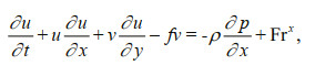
2.2 MethodThe spectral KE flux in SICC is calculated using high pass integral to momentum formula proposed by Frisch (1995, Chapter 2, Eq.2.52) and This method was applied by Scott and Wang (2005) to satellite altimeter dataset and reveal an inverse kinetic energy cascade in the South Pacific Ocean.
 (1)
(1) (2)
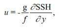
(2)where Frx and Fry are the frictional terms, including any vertical advection of the momentum. We begin with the horizontal momentum equations and velocity field can be estimated from the altimeter SSH data by assuming geostrophic:
 (3)
(3)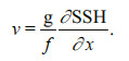 (4)
(4)where g is the gravity constant and f the Coriolis parameter. Meanwhile, EKE is calculated from the gridded SSH anomaly data SSH′ by assuming geostrophy: 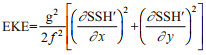
Here we assume a periodicity boundary condition. A linear tendency plane is removed from the selected 32×32 SSH field using least square method. Then, a Hanning window is set to the SSH field to reduce Gibbs effect for each grid in the study region. Fast Fourier transform (FFT) is used to get the information in the spectral space and calculate KE flux. The 32×32 window is big enough to capture the mesoscale spectral feature of altimeter data (Qiu et al., 2008; Tulloch et al., 2011; Wang et al., 2015).
Taking the FFT of Eqs.1 & 2, summing up these two equations after multiplying the equations in the Fourier space by the respective complex conjugates 
 (5)
(5)The forcing term P(kx, ky, t) arises from the vortexstretching term indicates the conversion of the available potential energy (APE) to KE. The Coriolis term dismissed because the Coriolis force is perpendicular to velocity, so there is zero work. In addition, the frictional terms became the dissipation term, D(kx, ky, t) in Eq.5. The spectral energy transfer term came from the horizontal nonlinear advection terms in Eqs.1 & 2:
 (6)
(6)where Δk=1/NΔx cycles per kilometer (cpkm), Δx is the grid spacing, and N is the number of grid points in the zonal of the meridional direction. The star indicates a complex conjugate while the caret and the horizontal curly bracket indicate fast Fourier transformation (FFT). As we take a 32×32 window, N=32 in this study for FFT. The horizontal wave number vector is (kx, ky)=2π(m/Lx, n/Ly), where m, n∈[-N/2, N/2]. The velocity field can be estimated from the altimeter SSH data by assuming geostrophy. For each window and each day, the SSH anomaly fields were first detrended by fitting a linear plane via least squares, and subtracting this plane from the corresponding day. A Hanning window was applied to the detrended data. The averages were over all available days and all boxes within the SICC band. T(kx, ky, t) indicates the EKE transfer between the different spatial modes, which is defined as KE transfer in this study.
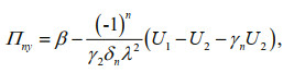
To determine the spectral KE flux П, we have defined the isotropic wave number as 

 (7)
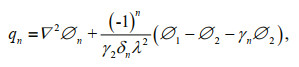
(7)By using a 2.5-layer reduced-gravity model (Qiu, 1999), the linearized governing equations are
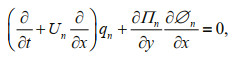 (8)
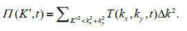
(8)where Ø n is the perturbation stream function, U1(U2) is the zonal mean velocity for SICC (SEC), and Πn is the mean potential vorticity. We assume the mean flow U n=const in meridional direction, qn and the meridional gradient of Πn are given by
 (9)
(9) (10)
(10)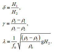 (11)
(11)In the above equations, Hn denotes the mean nth layer thickness, ρn the nth layer density, β the meridional gradient of the Coriolis parameter, f0 the Coriolis parameter basin mean at the reference latitude, and ρ0 the basin mean reference density.
The stability of this 2.5-layer reduced gravity SICC-SEC system can be analyzed by finding the normal-mode solution of Eq.8: 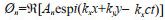
Scale analysis is applied to the spectral KE flux to distinguish two scales of different movements; inject and arrest scales. Inject scale (Scott and Wang, 2005), represents the spatial scale corresponding to the zero cross point with a positive slope in KE flux. At this scale, the KE injects into the system. On the other hand, arrest scale represents the start of arresting the energy and the presence of the minimum value of the KE flux. These scales are relevant to the observed energy-containing eddy scale through nonlinearity and can be used to evaluate the role of nonlinear physical process in eddy growth.
3 RESULT 3.1 Seasonal variation of EKE in SICCOur study shows that the monthly EKE variation based on 300-days high-pass filtered satellite altimeter data in the SICC region has distinct seasonal character, reaching a maximum of about 210 cm2/s2 in November, which is 1.5 times the minimum of about 140 cm2/s2 in May of the year (red line in Fig. 2). The filter is used to emphasize the contribution from the mesoscale eddy signals as the longest eddy life time is about 300 days. EKE seasonal variation indicates the existence of a growth-decay cycle of the eddy activity in SICC. The vertical shear of the mean zonal velocity (the geostrophic current accumulated from 1 500 m depth using WOA18 dataset) between 0–150 and 150–400 m layers reached its minimum of 3.1 cm/s every May and its maximum of 3.7 cm/s every November (Fig. 2, blue line) with the EKE. Despite synchronic growth and decline of the EKE and shear velocity, the shear velocity reached its maximum ahead of EKE by 1.5 months after May during the eddy growth phase (Fig. 2). The monthly variation of temperature gradient and velocity shear in the SICC has distinct seasonal character. Variation of the longitudinal temperature gradient and vertical velocity shear has synchronic character based on Thermal wind relationship.

|
| Fig.2 Monthly EKE variation in 1993–2016 (red line), vertical shear of zonal velocity (between 0–150 and 150–400 mean layers) (blue line), and meridional temperature gradient across 20°S upper 400 m (black dashed line) within two years in the SICC region Both temperature gradient and velocity shear have clear distinct seasonal cyclic character. |
To clarify the seasonal EKE evolution in SICC, the bimonthly EKE power spectral density (PSD) E (kx, ky, t) as a function of zonal and meridional wavenumber kx and kyis plotted in Fig. 3. We chose 9 points along 20°S on every 5° longitude from 65°E to 105°E as the centers of the boxes with 32×32 grid points. For each box daily, the SSH anomaly fields were first detrended by fitting a linear plane via least squares and subtracting this plane from its corresponding day. Hanning window was applied to the detrended data and the average values were obtained for all available days and boxes. As values on the edge of a Hanning window is close to zero, we set each window center inner the border of the nearby window as overlapping process to contain more information. The 9 boxes covered and contained the main information of the SICC basin and result is similar with equivalent 9 boxes along 25°S, which is reliable to reflect the basin scale characteristic.

|
| Fig.3 Bimonthly EKE power spectral density distributions as a function of kx and ky in the SICC band along 20°S, 60°E–110°E (shading, unit: m2/s2/cpkm/cpkm) The two-letter monthly designators started with October–November (ON, Fig. 3a) in the upper left and ended with August–September (AS, Fig. 3f) in the lower right. |
During the latest eddy growth phase of ON as the EKE continue to increase and reach to maximum (Fig. 2), the eddy signals have higher energy level at a large ky than at a large kx (Fig. 3a). This implies that energy in the kx-direction significantly increases with eddy growth. Meanwhile, EKE in DJ are notably distributed in the band with a larger spatial scale (i.e., smaller k) (Fig. 3b). Therefore, the EKE twodimension (2D) integral distribution is needed for further discussion. Here, we induced the method of Qiu et al. (2008) to identify the direction (zonal or meridional) where energy elongates more:
 (12)
(12) (13)
(13)where 
The most common practice in estimating the eddy length scale from SSH anomalies is the integral wave number of the isotropic kinetic energy spectrum. To quantitatively examine seasonal variations in the energy-containing eddy scale, following Qiu et al. (2008), we define
 (14)
(14)where 

|
| Fig.4 Monthly EKE variation (triangle markers) and eddy scale (rectangle markers) in 1993–2016 in SICC (a); zonally elongated EKE minus meridionally elongated (EKEz–EKEm)/EKE (b) |
The EKE in the SICC region was zonally elongated during the entire year and fairly agreed with the observed multi-zonal jets structure. The zonal elongation was the weakest in AS, whereas, it was strongest in FM. During ON, when the EKE level reached the seasonal maximum, zonal elongation preference of EKE in the 2D spectral domain in Fig. 3 started to increase, which is reflected in Fig. 4b through the (EKEz–EKEm)/EKE. The greater preference of EKE at larger zonal scales than at meridional scales continued in the subsequent months from February to September. Energy-containing eddy scale and EKE zonal elongation preference have consistent variation, which indicates stronger zonal elongation occurs as eddies grow larger. During the same period, there was a persistent drop in the overall energy level of mesoscale eddies until September when the EKE level started to increase together with large kx (Fig. 3).
3.2 Baroclinic instability and eddy growth phaseBy setting a seasonal cycle of the stratification and vertical shear of the zonal current, we used the 2.5-layer reduced-gravity model of Qiu (1999) to perform instability analysis. The two layers are 0–150 m and 150–400 m mean layers. Instability growth rate hasinverse correlation with the stratification term γ (


|
| Fig.5 Growth rate (/d) as a function of kx and ky for the SICC-SEC system in October–November (ON) (a), December– January (DJ) (b), February–March (FM) (c), April–May (AM) (d), June–July (JJ) (e), and August–September (AS) (f) (shading, unit: per day) Regions outside of the concentric circles are baroclinically stable. |
KE flux has a similar feature throughout the year in SICC. The KE flux in the scale, which is larger than the Rossby deformation radius, presents the characteristics of the inverse kinetic cascade (Fig. 6). This feature is similar with that in the South Pacific Subtropical Countercurrent (SPSTCC) area (Scott and Wang, 2005). Generally, the grid data accuracy of the satellite altimeter is considered to be more effective in the scale compared to the Rossby deformation radius. Based on the satellite altimeter data of 8 766 days, we calculated the regional KE flux mean of every grid point in the SICC region (18°S–30°S, 60°E–110°E) with each 32×32 window, obtaining a relatively smooth and statistically meaningful KE flux curve.

|
| Fig.6 Time-averaged spectral kinetic energy flux versus isotropic wavenumber (black line) in October–November (a), December–January (b), February–March (c), April–May (d), June–July (e), and August–September (f) in SICC calculated from 1993–2016 AVISO SSH The vertical red line is Karrest, and the vertical blue dashed line is the Kinject. |
A seasonal variation of the KE flux morphology, mainly in amplitude and length scale, is observed (Fig. 7). Particularly, the intensity of the KE flux significantly varied. The amplitude of the KE flux in February is obviously larger than that in August (Fig. 7). However, this seasonal variation of the KE flux has not been previously studied. The amplitude of the inverse kinetic cascade (blue shading) in the large scale, inject scale, and most unstable scale showed systemically seasonal cycle in SICC (Fig. 7). The amplitude reached its minimum in July, while the inject scale and most unstable scale reached its minimum in September. The inject scale lag the amplitude of the KE flux for about 3 months and is always larger by 30 km than that of the most unstable scale. In addition, a relatively weak direct kinetic cascade (Fig. 7, orange shading) started within the most unstable scale and transferred KE to the small scale.

|
| Fig.7 Monthly mean KE flux distribution of the SICC regional mean represented by the space shading (m2/s3) The black solid line is the monthly injection scale variation and the blue dash line is the most unstable scale calculated from 2.5-layer reduced gravity model. |
The monthly variations of the most unstable scale, arrest scale and energy-containing eddy scale in SICC have distinct seasonal characteristics that are nearly synchronically varying in phase. The highest values of about 154 km, 310 km, and 316 km respectively, were recorded in March and April, while the lowest values of about 130 km, 278 km, and 254 km respectively, were recorded in September (Fig. 8). The recorded minimum values in September of the year can be attributed to leading the maximum EKE in November by 2–3 months and corresponding to the months of the minimum zonal elongation of EKE PSD (Fig. 4b), indicating the correspondence between the minor KE flux arrest scale and less EKE zonal elongation.

|
| Fig.8 Monthly variation of the arrest scale in 1993–2016 (red line), energy-containing eddy scale (blue line), and the most unstable scale (black dashed line) within two years in the SICC region |
Figure 9 shows the bimonthly maps of the spectral transfer term T(kx, ky, t) as a function of zonal and meridional wavenumbers (kx, ky). 2D KE transfer shows the important role of KE in the energy transfer from most unstable length to energy-containing eddy scale captured by the satellite altimeter. The basic pattern of the KE transfer displays energy transfer path from the small and most unstable growth scales to the large and energy-containing eddy scale.

|
| Fig.9 Bimonthly distribution of the SICC regional mean KE transfer in cpkm (cycles per kilometer) wavenumber space (shading, unit: m2/s3/cpkm/cpkm) a. October–November (ON); b. December–January (DJ); c. February–March (FM); d. April–May (AM); e. June–July (JJ); f. August–September (AS). The large white circle refers to the isotropic most unstable scale calculated from 2.5-layer reduced gravity model while the small white circle refers to the isotropic eddy-containing eddy scale. |
Visually, the KE transfer is isotropic in most bimonths. However, KE transfer in eddy mature phase DJ bimonths illustrates notable characteristics from small scale to the zonal elongated large scale (Fig. 9b). Meanwhile, the initial turbulence preferred to begin within small meridional scales (Fig. 5), which suggests an anisotropic inverse cascade may transfer EKE from meridional elongated modes (kx>ky) to zonal elongated modes (kx < ky) when eddies grow large.
To investigate the anisotropy of the KE flux, we calculated the zonal and meridional spectral kinetic energy flux from T(kx, ky, t) in Fig. 9, respectively:
 (15)
(15) (16)
(16)The inverse cascade of Π x is detected in all months and may transfer energy to larger zonal scales. The zonal elongated KE flux Πx is especially deeper than the meridional elongated KE flux Πy above the inject scale (Fig. 10) in December. Meanwhile, the zonal elongated inverse kinetic cascade attenuated slower than that of the meridional elongated inverse kinetic cascade after reaching the arrest scale. Moreover, the zonal elongated inverse kinetic cascade continued to transfer kinetic energy to the barotropic (original) Rhines scale 

|
| Fig.10 Time-averaged spectral kinetic energy flux Π (black line) Πx is the zonal spectral kinetic energy flux (red line) and Πy is the meridional spectral kinetic energy flux (light blue line). |
The seasonality of the length scales and anisotropy of the KE transfer reflects the unique energy redistribution process in SICC. Qiu et al. (2008) reported that EKE in SPSTCC reached its maximum in October–November, which is the only bimonth period with meridional elongation of EKE 2D throughout the year. However, our result showed that EKE 2D elongation in SICC was zonal all year-round with more intensity, which differed from that in SPSTCC and is related to the observed notable multizonal jets in the study area (Menezes et al., 2014). The zonal elongation of EKE 2D in October– November in SICC is the weakest corresponding to the only meridional elongation of EKE 2D in SPSTCC (Qiu et al., 2008). We further found that synchronical seasonal variation of the inject, arrest and energy containing eddy scales, which lagged the physical quantities vertical shear of zonal velocity and meridional temperature gradient by 4–5 months. Moreover, the KE flux scale inclined to display the energy redistribution process.
The arrest and inject scales are located between the energy-containing eddy scale and most unstable scale. This can be explained as the bridge between the linear theory and practical observation. The arrest scale in SICC is about 300 km while the inject scale is about 150 km, which are close to that calculated values based on the monthly data in the SICC region (Tulloch et al., 2011; Wang et al., 2015). Chang and Oey (2014) suggested the energy-containing eddy scale is comparable to the largest eddy scale estimated by Chelton et al. (2011) from altimetry data. Meanwhile, these scales are close to the eddy diameter of 200 km from the eddy statistics in SICC obtained by Zheng et al. (2015) from surface drifters. The KE fluxes obtained based on the daily data were reserved and used to calculate the monthly mean result, which were used to calculate the inject and arrest scales for the corresponding month.
Our result of the KE transfer, especially the KE anisotropic transfer, is similar to that of previous studies (Qiu et al., 2008; Wang et al., 2015; Sérazin et al., 2018). Qiu et al. (2008) suggested that KE transfer might be related to 2D linear unstable circle band. However, we suggest that it is more reasonable to interpret the relationship between KE transfer with linear theoretic result and observation, since the ocean mesoscale process is highly nonlinear (Chelton et al., 2011). We further suggested that the negative value of the KE transfer responds the gap between the most unstable scale and energy-containing eddy scale, namely, the gap between linear and nonlinear process. The combination of KE linear and nonlinear process agrees to the KE path proposed by Smith and Vallis (2001) and the interpretation of the western boundary current proposed by Sérazin et al. (2018).
The amplitudes of KE in the inverse kinetic cascade with larger values than the radius of the Rossby deformation in the SICC region reached its maximum during summer, then subsequently gradually attenuated. The observed eddies are often not circular but have certain skewness. The result from the 2.5-layer model (Qiu et al., 2008) indicated instability in relatively small scale with notable meridionally elongated character in the 2.5-layer ocean structure of strong vertical shear of zonal velocity. However, the observed eddy energy in EKE PSD is distributed in the relatively large scale and has slightly zonal elongation throughout the year in SICC.
Despite the illustrated isotropic character of the KE flux in SICC, which differed from that in SPSTCC (Qiu et al., 2008), its skewness still seasonally varies. The anisotropy of the KE flux in SICC is mainly expressed in the large scale (Fig. 10), indicating the strongly inclination of KE to zonal elongation in December. The inverse cascade of zonal elongated KE flux Π x provides another possible explanation for the multi-zonal jets in the SICC region except the potential vorticity (PV) staircases model (Menezes et al., 2014).
The AVISO treated the data of the accuracy, completeness, and homogeneity (across time) of multiple satellites by merge and gridding process, and provides the daily data through interpolation. Although one week is needed for a single satellite to fly around the earth, however, the main current satellite data are formed based on the multiple satellite data. The instrumental errors in AVISO data are well corrected due to long-term observations and synthesis of track data of many satellites. However, there is some limitation in the effective identification of the spatial and temporal scales due to application of mesh and interpolation processes in the AVISO (Morrow and Le Traon, 2012; Wang et al., 2015). As we focused on mesoscale process in this study, AVISO data is reliable on both time and space resolution.
The KE flux calculation result of high-resolution models (Wang et al., 2015; Khatri et al., 2018) as in subtropical oceans showed that the shift of the flux to a smaller scale and the size reduction of the arrest scale. This is due to the influence of the grid resolution and interpolation process to the KE flux shape (Arbic et al., 2013). Moreover, the results from the models are linked with front instability, ageostrophic current and vertical velocity in North Pacific countercurrent (NPSTCC) (Qiu et al., 2014; Sasaki et al., 2017). They revealed that inverse kinetic cascade could extend to sub-mesoscale in high-resolution models and may transfer the submesoscale energy to larger scale and influence mesoscale variability. Chang and Oey (2014) found a faster growth rate in shorter wavelengths in NPSTCC, which implied the nonlinear process might be effective before perturbations to grow to mature phase. The length scale and anisotropy characteristic in the sub-mesoscale domain deserves further investigation. With this, the new Surface Water and Ocean Topography (SWOT) satellite altimeter scheduled to launch in 2021 is expected to provide some insights.
5 CONCLUSIONWe found that the isotropic length scale has seasonal variation. This scale is characterized by synchronic variation of the linear baroclinic most unstable scale and observed energy-containing eddy scale. This variation lagged EKE by 4–5 months indicates that the 2D redistribution process continues even the maximum 1D integrated physical quantity reached its maximum and followed by its declination, The negative value of the KE transfer is fully constrained by the linear most unstable scale and energy-containing eddy scale. The arrest and inject scales of the KE flux have collapsed within the baroclinic unstable and observed energy-containing eddy scales. Hence, KE transfer acts as a bridge among different scales, leveling further the gap between different spatial scales.
Temporal eddy energy redistribution process explained the 4–5-month lag in energy-containing eddy scale behind the regional EKE seasonal cycle caused by the 2D distribution skewness. The role of seasonal variation in systematic eddy energy redistribution process is further systema-tically interpreted, thereby providing another possible explanation for multi-zonal jets in the SICC region.
6 DATA AVAILABILITY STATEMENTThe altimeter products have been produced by DUACS with AVISO and distributed by CMEMS. Data could be downloaded from http://marine. copernicus.eu/. The product name is global ocean gridded L4 sea surface heights and derived variables reprocessed (1993-ongoing) and the identifier of product is SEALEVEL_GLO_PHY_L4_REP_ OBSERVATION_008_047. The World Ocean Atlas 2018 (WOA18) dataset is available at https://www. nodc.noaa.gov/OC5/woa18/woa18data.html.
7 ACKNOWLEDGMENTWe appreciate helpful discussion with Dr. LIU Chuanyu.
Arbic B K, Polzin K L, Scott R B, Richman J G, Shriver J F. 2013. On eddy viscosity, energy cascades, and the horizontal resolution of gridded satellite altimeter products. Journal of Physical Oceanography, 43(2): 283-300.
DOI:10.1175/jpo-d-11-0240.1 |
Chang Y L, Oey L Y. 2014. Instability of the North Pacific subtropical countercurrent. Journal of Physical Oceanography, 44(3): 818-833.
DOI:10.1175/Jpo-D-13-0162.1 |
Chelton D B, Schlax M G, Samelson R M. 2011. Global observations of nonlinear mesoscale eddies. Progress in Oceanography, 91(2): 167-216.
DOI:10.1016/j.pocean.2011.01.002 |
Delman A S, Lee T, Qiu B. 2018. Interannual to multidecadal forcing of mesoscale eddy kinetic energy in the Subtropical Southern Indian Ocean. Journal of Geophysical Research:Oceans, 123(11): 8.
DOI:10.1029/2018jc013945 |
Ferrari R, Wunsch C. 2010. The distribution of eddy kinetic and potential energies in the Global Ocean. Tellus A:Dynamic Meteorology and Oceanography, 62(2): 92-108.
DOI:10.3402/tellusa.v62i2.15680 |
Frisch U. 1995. :Turbulence:The Legacy of A. N. Kolmogorov. Cambridge University Press, Cambridge. 296ps.
|
Jia F, Wu L X, Lan J, Qiu B. 2011a. Interannual modulation of eddy kinetic energy in the southeast Indian Ocean by Southern Annular Mode. Journal of Geophysical Research:Oceans, 116(C2): C02029.
DOI:10.1029/2010jc006699 |
Jia F, Wu L X, Qiu B. 2011b. Seasonal modulation of eddy kinetic energy and its formation mechanism in the Southeast Indian Ocean. Journal of Physical Oceanography, 41(4): 657-665.
DOI:10.1175/2010jpo4436.1 |
Khatri H, Sukhatme J, Kumar A, Verma M K. 2018. Surface ocean enstrophy, kinetic energy fluxes, and spectra from satellite altimetry. Journal of Geophysical Research:Oceans, 123(5): 3 875-3 892.
DOI:10.1029/2017jc013516 |
Menezes V V, Phillips H E, Schiller A, Bindoff N L, Domingues C M, Vianna M L. 2014. South Indian Countercurrent and associated fronts. Journal of Geophysical Research:Oceans, 119(10): 6 763-6 791.
DOI:10.1002/2014jc010076 |
Morrow R, Le Traon P Y. 2012. Recent advances in observing mesoscale ocean dynamics with satellite altimetry. Advances in Space Research, 50(8): 1 062-1 076.
DOI:10.1016/j.asr.2011.09.033 |
Palastanga V, van Leeuwen P J, Schouten M W, de Ruijter W P M. 2007. Flow structure and variability in the subtropical Indian Ocean:Instability of the South Indian Ocean Countercurrent. Journal of Geophysical Research:Oceans, 112(C1): C01001.
DOI:10.1029/2005JC003395 |
Qiu B, Chen S M, Klein P, Sasaki H, Sasai Y. 2014. Seasonal mesoscale and submesoscale eddy variability along the North Pacific subtropical countercurrent. Journal of Physical Oceanography, 44(12): 3 079-3 098.
DOI:10.1175/Jpo-D-14-0071.1 |
Qiu B, Scott R B, Chen S M. 2008. Length scales of eddy generation and nonlinear evolution of the seasonally modulated South Pacific Subtropical Countercurrent. Journal of Physical Oceanography, 38(7): 1 515-1 528.
DOI:10.1175/2007jpo3856.1 |
Qiu B. 1999. Seasonal eddy field modulation of the North Pacific subtropical countercurrent:TOPEX/Poseidon observations and theory. Journal of Physical Oceanography, 29(10): 2 471-2 486.
DOI:10.1175/1520-0485(1999)029<2471:Sefmot>2.0.Co;2 |
Rhines P B. 1975. Waves and turbulence on a beta-plane. Journal of Fluid Mechanics, 69(JUN10): 417-443.
DOI:10.1017/s0022112075001504 |
Robinson A R. 1983. Eddies in Marine Science. Berlin, Heidelberg:Springer.
|
Sasaki H, Klein P, Sasai Y, Qiu B. 2017. Regionality and seasonality of submesoscale and mesoscale turbulence in the North Pacific Ocean. Ocean Dynamics, 67(9): 1 195-1 216.
DOI:10.1007/s10236-017-1083-y |
Scott R B, Wang F M. 2005. Direct evidence of an oceanic inverse kinetic energy cascade from satellite altimetry. Journal of Physical Oceanography, 35(9): 1 650-1 666.
DOI:10.1175/JPO2771.1 |
Sérazin G, Penduff T, Barnier B, Molines J M, Arbic B K, Müller M, Terray L. 2018. Inverse cascades of kinetic energy as a source of intrinsic variability:a global OGCM study. Journal of Physical Oceanography, 48(6): 1 385-1 408.
DOI:10.1175/jpo-d-17-0136.1 |
Smith K S, Vallis G K. 2001. The scales and equilibration of Midocean eddies:freely evolving flow. Journal of Physical Oceanography, 31(2): 554-571.
DOI:10.1175/1520-0485(2001)031<0554:tsaeom>2.0.co;2 |
Tulloch R, Marshall J, Hill C, Smith K S. 2011. Scales, growth rates, and spectral fluxes of baroclinic instability in the ocean. Journal of Physical Oceanography, 41(6): 1 057-1 076.
DOI:10.1175/2011jpo4404.1 |
Wang S H, Liu Z L, Pang C G. 2015. Geographical distribution and anisotropy of the inverse kinetic energy cascade, and its role in the eddy equilibrium processes. Journal of Geophysical Research:Oceans, 120(7): 4 891-4 906.
DOI:10.1002/2014jc010476 |
Wunsch C. 1997. The vertical partition of oceanic horizontal kinetic energy and the spectrum of global variability. Journal of Physical Oceanography, 27(8): 1 770-1 794.
DOI:10.1175/1520-0485(1997)027<1770:tvpooh>2.0.co;2 |
Zheng S, Du Y, Li J, Cheng X. 2015. Eddy characteristics in the South Indian Ocean as inferred from surface drifters. Ocean Science, 11(3): 361-371.
DOI:10.5194/os-11-361-2015 |