 2020, Vol. 38
Institute of Oceanology, Chinese Academy of Sciences
Article Information
- GENG Wu, CHENG Feng, XIE Qiang, ZOU Xiaoli, HE Weihong, WANG Zhaozheng, SHU Yeqiang, CHEN Gengxin, LIU Danian, YE Dong, WANG Ruiwen, LIU Chuanyu
- Observation system simulation experiments using an ensemble-based method in the northeastern South China Sea
- Journal of Oceanology and Limnology, 38(6): 1729-1745
- http://dx.doi.org/10.1007/s00343-019-9119-4
Article History
- Received May. 7, 2019
- accepted in principle Jun. 25, 2019
- accepted for publication Oct. 30, 2020


2 China General Nuclear Power, Yangjiang Nuclear Power Co., Ltd., Yangjiang 529941, China;
3 Laboratory for Regional Oceanography and Numerical Modeling, Qingdao National Laboratory for Marine Science and Technology, Qingdao 266071, China;
4 Institute of Deep-sea Science and Engineering, Chinese Academy of Sciences, Sanya 572000, China;
5 Center for Ocean Mega-Science, Chinese Academy of Sciences, Qingdao 266071, China;
6 Public Weather Service Center of China Meteorological Administration, Beijing 100081, China;
7 National Meteorological Center of China Meteorological Administration, Beijing 100081, China;
8 Key Laboratory of Ocean Circulation and Waves, Institute of Oceanology, Chinese Academy of Sciences(IOCAS), Qingdao 266071, China;
9 Marine Dynamic Process and Climate Function Laboratory, Pilot National Laboratory for Marine Science and Technology(Qingdao)(QNLM), Qingdao 266237, China
Kuroshio is the strongest western boundary current (WBC) in the Pacific. When passing by the Luzon Strait (LS), most of the Kuroshio water flows out of the LS through a looping path, while some of it intrudes into the South China Sea (SCS; Yuan et al., 2006; Chen et al., 2011a; Nan et al., 2011a; Shu et al., 2018a), and leads to complex circulations (Qu et al., 2004; Nan et al., 2011a; Wu and Hsin 2012; Shu et al., 2016a, 2018b) and energetic eddy activities in the northeastern SCS (Fig. 1; Wang et al., 2008a; Chen et al., 2011b; Nan et al., 2011b; Liu et al., 2012b; Shu et al., 2016b; Chu et al., 2017). The spatial patterns and temporal variability of the circulations and mesoscale processes are crucial to local marine environment and air-sea interactions, thus becoming one of the hot research topics (Xian et al., 2012; Zhang et al., 2013; Guan et al., 2014; Huang et al., 2014). However, our knowledge of the variability in the northeastern SCS is still limited due to the lack of observations. Recently, a large number of observations have been collected in the northeastern SCS by different researchers (Tian et al., 2006; Chen et al., 2010, 2011a, c; Yang et al., 2010a, 2015); however, continuous observations are rare. It is worth noting that some researchers have carried out continuous observations in the northeastern SCS. Ocean University of China designed and placed 18 mooring arrays in the northeastern SCS, and parts of station data were used in several studies (Fig. 2; Zhang et al., 2013; Guan et al., 2014; Huang et al., 2014). The mooring array has successfully documented a pair of deep-penetrating mesoscale eddies that generated southwest of Taiwan, China, and could greatly influence the deep circulation in the northeastern SCS (Zhang et al., 2013). Continuous observations always have two goals: one is to capture the potential physical phenomena in the ocean; another is to assimilate the observation results to improve the model simulation. Before assimilating the observation results to the model, designing a suitable observing system is necessary. However, the design of such an observation system as shown in Fig. 2 is based typically on empirical knowledge, rather than quantitative assessments. For the high costs involved in building and maintaining the observing system, designing and optimizing an observing system are necessary; and an observation system simulation experiment (OSSE) is a possible solution to this problem. An OSSE can be used to determine the potential benefit of future observing systems using an existing monitoring system; it help define optimal characteristics of future instruments and evaluate the present sampling distribution, and optimize construction design, and shall play a key role in developing an ocean observing system (Smith, 1993; Sakov and Oke, 2008).

|
| Fig.1 A sketch of different types of Kuroshio intrusions Adapted from Caruso et al. (2006). Type 1 (grey) shows the mean position of the Kuroshio; Type 2a (thick, solid) shows the SCS Branch of the Kuroshio; Type 2b (short dashed) is an anticyclonic loop current; Type 2c (long dashed) is an anticyclonic eddy that has detached from Type 2b intrusion; Type 3 (thin, solid) enters in the northern part of the Luzon Strait and forms a cyclonic circulation. The blue (red) line represents the position of the Luzon cyclonic gyre (LCG) in winter (summer), and the pink line represents the position of Luzon cyclonic eddy (LCE) (Fang et al., 1998). |

|
| Fig.2 Water depth (units: m) of the study region and distribution of the 18 present in-situ stations (mooring stations) The black line represents the nine-dash line. |
Based on the data assimilation theory, the OSSE, which was originally used in meteorology (Charney et al., 1969) had been widely employed to design observing systems for the world's oceans (Hackert et al., 1998; Bishop et al., 2001; Hirschi et al., 2003; Schiller et al., 2004). Especially, in the tropical Indian Ocean (TIO), there were many applications of the OSSE to assess the ability of the monitoring system (Ballabrera-Poy et al., 2007; Oke and Schiller, 2007; Vecchi and Harrison, 2007; Sakov and Oke, 2008). Some applied the OSSE to place and optimize stations in coastal waters (Frolov et al., 2008; Yildirim et al., 2009; Xue et al., 2011, 2012). Others focused on designing the optimal monitoring sites for biological oceanography research (Lin et al., 2010; Xue et al., 2011, 2012). Varieties of methods have been introduced to the framework of OSSE, which extended the efficiency of OSSE in assessing the ability of observation systems. Using an empirical orthogonal function (EOF) and data assimilation method, a mooring array had been designed and evaluated to monitor the intraseasonal and interannual variability in the TIO (Ballabrera-Poy et al., 2007; Oke and Schiller, 2007; Vecchi and Harrison, 2007; Sakov and Oke, 2008). EOF-based approach was also employed by Yang et al. (2010b) to select the optimal sensor locations for noisy ocean measurements in the Nantucket Sound. A variance quadtree (VQT) algorithm for optimizing survey design was developed by McBratney et al. (1999) and improved by Minasny et al. (2007). Lin et al. (2010) used the VQT algorithm to have optimized plankton survey strategies in the Gulf of Maine. Based on a high-resolution ocean model, some researchers carried out the OSSE using the ensemble Kalman Filter (EnKF) data assimilation approach (Evensen, 2003, 2004; Chen et al., 2009; Xue et al., 2011, 2012; Liu et al., 2018a). According to the Kalman Filter theory, a simplified and computationally efficient, ensemble-based method for OSSE (hereafter EnOSSE) was introduced by Bishop et al. (2001), and had been used intensively for optimal array design in the last few years (Khare and Anderson, 2006; Sakov and Oke, 2008; Ye and Wang, 2011; Wang and Ye, 2012; Liu et al., 2018b). This method is used to design an optimal array based on an ensemble system state, which may come from model results or from long time series of field observations. Sakov and Oke (2008) used the long time series of sea level anomaly (SLA) data from satellite altimeter to design an optimal array to monitor the intraseasonal to interannual variability in the TIO.
There also exists intraseasonal to interannual variations in the northeastern SCS. The Kuroshio intrusion has significant intraseasonal variability (10–30 days and 60 days), the 10–30 days variability is caused by the high-frequency variability of local winds and the baroclinic instability, whereas the 60 days cycle is mainly for the intrusion of eddies (Zhang et al., 2015). The Kuroshio path in the LS also has seasonal variability for the mesoscale eddies and monsoons (Shaw, 1991; Yuan and Li, 2008; Nan et al., 2011a; Yuan and Wang, 2011). The interannual variability of Kuroshio intrusion into the SCS is mainly caused by the El Niño-Southern Oscillation (ENSO; Qu et al., 2004; Liu et al., 2006, 2012a). Some researchers focused on the intraseasonal variability in upwelling intensity in the northern SCS (Shu et al., 2011; Wang et al., 2012; Gan et al., 2015); the upwelling in the northern SCS also has strong interannual variability (Jing et al., 2011; Shu et al., 2018b). About the mesoscale eddies, Chen et al. (2011b) pointed out that the number, radius and lifetime of the eddies have seasonal and interannual variability in the northern SCS. The Luzon cyclonic gyre (LCG) also has strong seasonal variability for the monsoons (Fig. 1; Fang et al., 1998; Gan et al., 2006). Controlled by the monsoons, Kuroshio intrusion and other factors, the circulation and mesoscale eddies in the northeastern SCS present a complex intraseasonal to interannual variations (Su, 2005). Therefore, it is necessary to design an array to monitor the intraseasonal to interannual variations in the northeastern SCS.
Although OSSEs have been used widely for promoting monitoring efficiency in the world's oceans, few applications have been conducted to design and assess a stationary observation network in the northeastern SCS. Therefore, detailed studies for quantitatively examining the present stations' distribution and constructing an optimal observation system are necessary. Furthermore, previous studies usually focused on optimal station distribution in horizontal direction, while the optimal vertical distribution of observation instruments, i.e., which layers play more key roles to the observing system, was often ignored. However, when building and maintaining a stationary mooring array to monitor the current, we always need to synchronously place dozens of observation instruments and monitor units (such as conductivity-temperature-depth (CTD) machine) in different layers. To promote monitoring efficiency and to be more economical, studying optimal vertical layers is also required.
In this study, we first focus on the design of an optimal array and quantitative evaluation of the present in-situ stations using the ensemble-based method for OSSE in the northeastern SCS. Then, we quantitatively examine the performance of observations in different layers and find the optimal design in the vertical. This paper is organized as follows. In Section 2, we briefly describe the method. In Section 3, we introduce the data to be analyzed. Our results are presented in Section 4, and the summary is given in Section 5.
2 METHODThe EnOSSE (Bishop et al., 2001; Sakov and Oke, 2008) is applied in the present study. Assuming that the uncertainty of a state vector Xn×l can be represented by a background error covariance matrix Pb, which is expressed as follows:
 (1)
(1)where A is the anomaly field of the state vector Xn×l and can be defined as 
According to the Kalman Filter theory (Evensen, 2003, 2004), after assimilating a set of observations, the background error covariance matrix Pb is updated, which can be represented by
 (2)
(2)where Pa is the updated Pb, K is the Kalman Gain defined as follows:
 (3)
(3)R in Eq.3 is the observational error covariance. H is an observation matrix that projects the model data onto the observational points, if assimilating q observations, H is given as Hq×n, when q=1, 
 (4)
(4)According to the relation trace(AB)=trace(BA), the solution of Eq.4 can be described by
 (5)
(5)When searching for the first optimal observational site, H in Eq.5 becomes 1×n vector, replacing Pb in Eq.5 with that in Eq.1. Then, we get the first optimal observational site k, which can be written as follows:
 (6)
(6)where Ai is the ith row of A. After finding the first optimal observation, we update Pb with Eq.2, and then calculate the next optimal observation; and Pb is updated again, until all q optimal observations are found. When n≫m, directly manipulating the matrix Pb with a dimension n×n in Eq.2 is very difficult, so a computationally effective solution is given by Bishop et al. (2001), replacing directly updating Pb in Eq.2 by updating the background ensemble Ab as follows:
 (7)
(7) (8)
(8)In the above equations, I is the identity matrix, 
 (9)
(9)where U is an orthogonal matrix and Λ is a diagonal matrix. Then, T can be written as
 (10)
(10)The above method tells us how to find an optimal array, or how to get the optimal set of observation matrix Hopt. When evaluating the present in-situ stations (Fig. 2), the observation matrix H is known, and then the background ensemble Ab can be updated using Eqs.7–10, which leads to the updating of Pb in Eq.1. According to the Kalman Filter theory, the background error covariance matrix Pb characterizes the uncertainty of the initial ensemble, so we can assess the ability of the present observing system according to the updating of Pb.
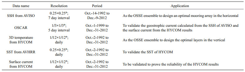
3 DATAThe present in-situ stations were designed to monitor the current and eddy activities in the northeastern SCS (Zhang et al., 2013; Guan et al., 2014; Huang et al., 2014). In this study, a long time series of sea surface height (SSH) from satellite altimeter were employed to construct the ensemble to represent the variability of the current and eddy activities. The weekly SSH data from the AVISO (Archiving, Validation and Interpretation of Satellite Oceanographic data) is from Oct.-14-1992 to Dec.-9- 2012. The AVISO product combines data from multiple satellites, including TOPEX/Poseidon, Jason-1, the European Remote Sensing (ERS) Satellites 1, 2 and their successor (Ducet et al., 2000). It has a resolution of 0.25°, the detailed information of the data used in this paper can be found in Table 1. SSH samples can reflect the intraseasonal to interannual variability of the geostrophic current of the study domain. To better understand the variability of the current, we compare the geostrophic currents from the AVISO and the surface currents from the Ocean Surface Current Analysis-Real Time (OSCAR). The OSCAR product is available beginning from October 1999, with a horizontal resolution of 1/3° and 5-day interval (Table 1; Bonjean and Lagerloef, 2002; Johnson et al., 2007), and represents the ocean current (both geostrophic and Ekman components) of the upper 30 m. The temporal resolution of OSCAR and AVISO data are 5-day and 7-day, respectively, to compare the two data, we linearly interpolate the OSCAR and AVISO data into 1-day interval. Figure 3 is the time series of the surface current from OSCAR and the surface geostrophic current from AVISO at station H in Figs. 4 & 5a where the SSH has the largest root-meansquare 


|
| Fig.4 The distribution of correlation coefficients between the time series of u component from OSCAR and AVISO during January 1999–December 2012 (a); same as (a), except for the v component (b) The station H is located at the position where SSH of AVISO has the largest RMS. The black line represents the nine-dash line. |

|
| Fig.5 The distribution of RMS (units: cm) of SSH from AVISO (a) and RMS (units: ℃) of SST from HYCOM (b) T he station H and T are located at the position where SSH and SST have the largest RMS, respectively. The black line represents the nine-dash line. |
Due to the lack of large number of threedimensional (3D) observations in the northeastern SCS, 3D weekly temperature results from the HYCOM global 1/12° reanalysis products (Table 1; Experiments 19.0 & 19.1; Fox et al., 2002; Cummings, 2005; Cummings and Smedstad, 2013) are used to evaluate the optimal sampling deployment in the vertical. The HYCOM has a high resolution of 1/12° in the horizontal, and contains 32 hybrid layers in the vertical. The surface forcing of the model is from hourly National Centers for Environmental Prediction (NCEP) Climate Forecast System Reanalysis (CFCR) products, including wind stress, heat fluxes, and precipitation. To improve the forecast capability of both temperature and salinity, a 3D variational algorithm is used to assimilate available satellite altimeter observations, in-situ sea surface temperature (SST) and available in-situ vertical temperature and salinity profiles from XBTs, Argo floats and moored buoys. The HYCOM results exhibit a flow pattern similar to the observations in the LS (Zhang et al., 2010; Zeng et al., 2018), it also reproduces the variation in the Kuroshio intrusion reasonably well on both seasonal and interannual scales (Nan et al., 2011a; Yuan et al., 2014). By comparing the monthly T-S diagram of the HYCOM results with that of the observations, Wang et al. (2015) suggested that the model reproduces the monthly temperature and salinity profiles well in the northeastern SCS. Using the in-situ temperature profiles with different sources in the northeastern SCS, Lian et al. (2019) proved the reliability of the HYCOM results in the northeastern SCS. The weekly temperature results used in this study are from Oct.-2-1992 to Dec.-31-2012. To promote computational efficiency of determining the optimal sampling deployment in the vertical, we only consider the sampling deployment in the surface and middle layers of the ocean, so the 3D temperature data of 19 standard layers (0, 10, 20, 30, 50, 75, 100, 125, 150, 200, 250, 300, 400, 500, 600, 700, 800, 900, 1 000 m) are employed in this study.
To validate the representation skill of the HYCOM reanalysis products, we compare the SST from HYCOM with that of the Advanced Very High Resolution Radiometer (AVHRR). The AVHRR product has the longest record (from late 1981 to the present) of SST measurements from a single sensor design (Table 1). Infrared instruments, like AVHRR, can make observations at relatively high resolution but cannot see through clouds. The daily SST from AVHRR used here is an analysis product that has a spatial resolution of 0.25° (Banzon et al., 2016). Figure 6 depicts the time series of SST from HYCOM and SST from AVHRR at station T where SST from HYCOM has the largest RMS (Fig. 5b). The results show that the SST from HYCOM at station T agrees very well with that of AVHRR (the correlation coefficient is up to 0.98). Figure 7 is the distribution of correlation coefficients between the SST time series from HYCOM and AVHRR from Oct.-2-1992 to Dec.-31-2012, we can see that the SST from HYCOM is also very well consistent with that of AVHRR, the mean correlation coefficient in the study area is up to 0.96. Therefore, we can conclude that the temperature data from HYCOM is suitable to represent the intraseasonal to interannual variation in the northeastern SCS.

|
| Fig.6 Time series of SST from HYCOM and AVHRR at station T from Oct.-2-1992 to Dec.-31-2012 The station T is shown in Fig. 5b where SST from HYCOM has the largest RMS. |

|
| Fig.7 The distribution of correlation coefficients between the SST time series from HYCOM and AVHRR from Oct.- 2-1992 to Dec.-31-2012 T he station T is located at the position where SST of HYCOM has the largest RMS. The black line represents the nine-dash line. |
Because geostrophic balance is dominant in this region (Figs. 3–4), the surface current is proportional to the SSH gradient which reflects the vertical structures. To further validate the representation skill of the HYCOM reanalysis products, it is necessary to validate the surface current of HYCOM (Table 1). Figure 8 is the time series of the surface current from OSCAR and HYCOM at station H. Because we focus on the weekly temperature products from HYCOM, the high-frequency variability of the surface current from HYCOM within 7 days is filtered. As shown in Fig. 8, although the surface current from HYCOM is larger than that of OSCAR, the two datasets are consistent in terms of phase. The correlation coefficients of the u and v components between the two datasets are 0.69 (Fig. 8a) and 0.57 (Fig. 8b), respectively. The distribution of correlation coefficients between the time series of u and v components from OSCAR and HYCOM also indicates that the small correlation coefficient only appears at a small area, while the large value appears at a large area (Fig. 9), which again proves the reliability of the HYCOM results.

|
| Fig.8 Same as Fig. 3, except for the time series of the surface current from OSCAR and HYCOM at station H |

|
| Fig.9 Same as Fig. 4, except for the distribution of correlation coefficients between the time series of u (a) and v (b) components from OSCAR and HYCOM The black line represents the nine-dash line. |
To improve the accuracy of the optimal stations' locations, we remap SSH data to the high-resolution grid of the HYCOM results (SSH data from AVISO is bilinearly interpolated into the HYCOM grid). The SSH data within water depth of 150 m are discarded due to the bad quality of offshore altimetry data. This is also applied to the 3D temperature ensemble to maintain consistency of the study domain, which is shown in Fig. 2. The number of variables (n)/samples (m) for the SSH and 3D temperature datasets are 5 131/1 052 and 92 066/1 050 in this study, respectively.
4 RESULT 4.1 SSH ensemble resultsSSH is selected as the ensemble to design an optimal array and assess the present in-situ stations in the northeastern SCS in this study. We assume that SSH has an error variance R of 4, 9, and 16 cm2, respectively, to discuss the relation between R and the distribution of optimal stations. The EnOSSE method is used to design the optimal array. When assimilating each optimal station, the initial Pb is updated, which leads to decreasing of the variance of the initial ensemble. A decrease in variance means less uncertainty in the initial sample.
As shown in Fig. 10, the mean SSH (MSSH; the MSSH is calculated from the study period in this paper (from Oct.-14-1992 to Dec.-9-2012)) has large values along the main axis of the Kuroshio in the LS and small values in the southwest of the study domain. The RMS of SSH has two large cores. The largest core is located at the west of LI where the LCG and Luzon cyclonic eddy (LCE) are energetic (Fig. 1; Fang et al., 1998; Gan et al., 2006); another large core is located at the northwest of the LS, where a large number of eddies are generated locally (Yuan et al., 2007; Wang et al., 2008b) or shed from the Kuroshio (Caruso et al., 2006; Yuan et al., 2006; Wang et al., 2008a; Nan et al., 2011a). For the three different error variances R, the first five optimal stations are almost located at the same locations. However, the locations of the subsequent optimal stations vary greatly with different R. The first optimal station is located at the northwest of LI, near the core of the largest RMS, where the energetic LCG occurs (Fig. 10). In winter, the LCG develops very well under the northeasterly monsoon, and dominates the flow pattern in the northeastern SCS, but it is greatly reduced by the southwesterly monsoon in summer (Fig. 1; Fang et al., 1998; Gan et al., 2006). The large seasonal variation of the LCG leads to a large RMS there, which needs more attention when we design an observing system; so, the first optimal station is reasonable. The 2nd and 4th optimal stations are at the edge of the LCG. The 3th optimal station is located at the northwest of the LS, where the Kuroshio path changes strongly, and a large number of mesoscale eddies can be found, leading to the second largest RMS of SSH (Fig. 1; Yuan et al., 2006; Zhuang et al., 2010; Nan et al., 2011a; Zu et al., 2013). The 5th optimal station is located at the southwest of Taiwan, China, which is energetic due to both Kuroshio loop current and eddy activities, especially the anticyclonic eddies (Nan et al., 2011a; Zu et al., 2013). We notice that the first five optimal stations all appear west of the LS due to the strong variation of currents and eddy activities. In contrast, the Kuroshio is stable east of the LS, only the 12th optimal station when R=4 and 9 cm2 and the 11th optimal station when R=16 cm2 can be found there.

|
| Fig.10 The optimal observation stations based on SSH ensemble with an error variance R of 4 cm2 (a), 9 cm2 (b), and 16 cm2 (c), respectively The numbers represent the ranking of individual locations. The white contours represent the MSSH (unit: cm), the shaded areas represent the RMS (unit: cm) of SSH. The pink line represents the nine-dash line. |
After assimilating all the 18 optimal stations, the basin-averaged RMS of the sample ensemble drops sharply to 3.09, 3.52, and 3.97 cm when R=4, 9, and 16 cm2, respectively (Fig. 11a), of which the first optimal station contributes most to the reduction, up to 2.71, 2.61, and 2.49 cm, respectively (Fig. 11b). It means that the northwest of LI is the key region. The first five stations reduce the basin-averaged RMS by 4.66, 4.47, and 4.24 cm when R=4, 9, and 16 cm2, respectively, accounting for about 65%, 67%, and 68% of the total reduction (Fig. 11a), which shows that the first five stations reduce the RMS considerably and all subsequent stations result in only very small further reduction. So, the first five optimal stations are most valuable, and should receive more attention when we design an observing system for the domain. Sakov and Oke (2008) pointed out that the locations of the optimal stations were determined not only by the variance of the ensemble, but also by the error variance R; however, they did not further discuss the relation between the error variance R and the RMS of the system. Figure 11a suggests that the RMS decreases faster if the error variance R is smaller. A smaller R represents a more accurate sample ensemble; so, the results show that if a more accurate sample ensemble is used to design an observing array, the same number of optimal stations can yield better observation results.

|
| Fig.11 The basin-averaged (a) and reduction (b) of RMS of SSH ensemble after assimilating the first n optimal stations and the nth optimal station, respectively |
We now set the observation matrix H to evaluate the present in-situ observation stations shown in Fig. 2. We set H1×n for different stations and assimilate each station for one cycle, and then assess the performance of each station. First, the results again indicate that each station will reduce the RMS much more; in other words, perform better if the error variance R is smaller (Fig. 12). Second, based on the SSH ensemble, the 18th station is most close to the core of the largest RMS of SSH (Fig. 10) and performs the best, with the basin-averaged RMS dropping by 2.62, 2.51, and 2.38 cm for R=4, 9, and 16 cm2, respectively, after assimilating this station for one cycle. The 4th station is also near the core of the largest RMS, so it also performs well. The 7th station, which can only reduce the basin-averaged RMS by less than 0.8 cm (Fig. 12), performs the worst. The results imply that the 18th and 4th present stations may have a different spatial correlation scale with the other insitu stations, so a correlation analysis is used next to address this problem.

|
| Fig.12 Reduction of RMS of SSH ensemble after assimilating the present nth station for one cycle |
We define Ci as the mean correlation coefficient (MCC) at the ith variable to the entire computational domain as follows,
 (11)
(11)where n is the total variables in the study domain, Corr(i, k) is the correlation coefficient of SSH for the ith and kth variables.
Figure 13 is the distribution of the MCC calculated using the SSH ensemble. It shows that the MCC of SSH is large in the northwest of LI and has a small value in the southwest of Taiwan, China, where the 7th station is located. The 18th station is located in the area where the MCC of SSH has a relative large value of 0.57 (Fig. 14); it means that the SSH there is well correlated with that of the entire domain. Therefore, the 18th station performs the best among all the 18 present stations based on the SSH ensemble. The SSH of the 7th station is relatively uncorrelated with that of the entire domain (Fig. 14), which explains why this station performs the worst. The 12th to 16th stations are located at the northwest of the LS, and are all hardly correlated with that of the entire domain, which explains why these stations receive the same small level of assimilation effect (Figs. 13–14). Therefore, we conclude that the present observing system may over sample at the northwest of the LS. Note that the tendency of the MCC for SSH ensemble in Fig. 14 is consistent with that of the reduction of RMS in Fig. 12. This implies that when evaluating an observing system based on certain sample ensemble, if a station is well (badly) correlated with the entire domain, it will reduce the RMS of the initial ensemble much more (less) after assimilating, leading to a good (bad) performance of this station.

|
| Fig.13 Distribution of the MCC calculated using SSH ensemble The black line represents the nine-dash line. |

|
| Fig.14 MCC of the nth present station |
To further evaluate the performance of the 18 present stations, we compare the capability of the present and optimal stations to reduce the RMS of the ensemble. In this case, we set R=9 cm2, and the results are shown in Fig. 15. The basin-averaged RMS of the initial SSH ensemble decreases gradually after assimilating no matter the optimal stations or present stations, and the optimal stations always perform better than the present stations. Assimilation of the first optimal station and the first present station, the basin-averaged RMS sharply drops to 7.64 and 8.94 cm, respectively. Later, the RMS drops more slowly after assimilating the subsequent stations. The RMS decreases to 3.52 and 5.10 cm after assimilating all the 18 optimal and present stations, respectively. It implies that the future observation stations of the same number, if they are in the key regions as revealed above, can receive better observation effects. We notice that the basin-averaged RMS of SSH ensemble decreases slightly after assimilating the present stations from the 12th to 16th stations, it also implies that the present observing system may over sample from the 12th to 16th stations.

|
| Fig.15 The basin-averaged RMS of SSH ensemble after assimilating the first n optimal and present stations |
Now, we investigate the horizontal distribution of the RMS after assimilating all the 18 stations (R=9 cm2). The results are shown in Fig. 16. We can see that small RMS only appears at a small area around the present stations, while big RMS appears within a large area of the southwest of the study domain (Fig. 16a). This suggests that the present stations only perform well in a small surrounding area, while performing badly at the southwest of the study domain, implying that the present observing system may under sample there. On the contrary, for the optimal stations, small RMS occurs in most of the domain (Fig. 16b), indicating that the optimal stations perform well in most of the domain. Figure 17 is the proportion of the area less than different RMSs after assimilating all the 18 optimal and present stations. The area ratio of the RMS < 3 cm is no more than 22% for assimilating of either the 18 optimal or present stations, implying that the optimal stations perform almost the same as the present stations at this level. It shows that the optimal and present stations all perform best within a small region. With the increase of the RMS, the difference of the area ratio at the optimal and present stations becomes larger and larger, and reaches its maximum, up to 47% at RMS=4.5 cm (the optimal and present stations could reduce the RMS of about 94% and 47% of the domain to less than 4.5 cm, respectively). This indicates that the optimal stations perform better for a larger area.

|
| Fig.16 Horizontal distributions of RMS (units: cm) of SSH ensemble after assimilating all the 18 present (a) and optimal (b) stations The black line represents the nine-dash line |

|
| Fig.17 Area ratio that is less than certain RMS after assimilating all 18 optimal and present stations |
Previous research often focused on designing an optimal observing array in the horizontal to monitor the current; few concerns were made about the vertical distribution of observation instruments (such as the CTD machine). To promote observing efficiency and be more economical, the study of determining optimal layers is of the same importance. The 3D weekly temperature at 19 standard levels from the HYCOM global 1/12° reanalysis products are used as the sample ensemble here. We treat all the temperature data in different layers as the samples. Unlike the 2D SSH ensemble, which has only n computational variables (Eq.11; the SSH ensemble has n=5 131 variables), the temperature ensemble used here has close to 19×n computational variables, which requires more computational cost (the water depth is no more than 1 000 m in some regions, leading to less than 19 temperature data in the vertical there).
Based on the EnOSSE method, three different error variances (see below) are set to determine the optimal position in the vertical. Note that in this subsection we mainly focus on the vertical distribution of the first 18 optimal layers, so that the horizontal distribution of the optimal stations is not shown or discussed. As shown in Fig. 18a, when R=0.04, 0.25, and 0.64 (℃)2, the first optimal layer is 20 m, 20 m and surface, respectively. Furthermore, for different R, all the 18 optimal layers are located within the upper 200 m, meaning that placing observation instruments and monitoring factors within the upper 200-m depth is more important for the observing system. After assimilating all the 18 optimal layers, the basinaveraged RMS is decreased sharply to 0.48, 0.52, and 0.57℃ when R=0.04, 0.25, and 0.64 (℃)2, respectively, of which the first optimal layer contributes most to the reduction, up to 0.37, 0.34, and 0.31℃, respectively (Fig. 18b). This indicates the surface and subsurface layers reduce the RMS considerably and thus are most valuable.

|
| Fig.18 Vertical distribution of the nth optimal station (a); same as Fig. 11a, except for the 3D temperature ensemble (b) |
The ensemble-based method for OSSE is employed to design the optimal stations and assess the present stations in the northeastern SCS. To monitor the intraseasonal to interannual variability in the northeastern SCS, the SSH from the satellite altimeter is treated as the initial sample ensemble to discuss the horizontal distribution of the optimal stations.
Based on the SSH ensemble, our results show that the most key region is located at the northwest of LI, where SSH has a very large RMS and the energetic LCG occurs. Other key regions are near the edge of the LCG, at the northwest of the LS and the southwest of Taiwan, China. The first five optimal stations account for more than 65% of the total reduction of the RMS, of which the first optimal station contributes most to the reduction; it shows that the first five stations are most valuable. We further discuss the relation between the error variance R and the RMS of the ensemble. These results suggest that the basinaveraged RMS decreases faster if the error variance R is smaller. A smaller initial R means a more accurate initial sample ensemble, so these results imply that if the optimal stations are designed based on a more accurate and representative initial sample ensemble, the same number of stations can yield better observation effects.
For the present in-situ stations, our results indicate that the 18th (7th) station performs the best (worst) (Fig. 12). The 12th to 16th stations perform badly, and we conclude that the present observing system may over sample at the northwest of the LS. Only the 4th and 18th stations are close to the key region where the energetic LCG occurs (Figs. 10 & 13); so, we conclude that the present observing system may under sample at the northwest of LI. To explain these results, correlation analysis is employed. We show that the 18th station is located in the area where the MCC of SSH is very large (Fig. 13), which means that the SSH there is well correlated with that of the entire domain. Therefore, the 18th station performs the best among all 18 present stations. The MCC of SSH has a very small value at the southwest of Taiwan, China, where the 7th station is located (Fig. 13); it means that the SSH of this station is relatively uncorrelated with that of the entire domain, which leads to the worst performance of the 7th station.
We further compare the capability of present and optimal stations to reduce the basin-averaged RMS of the ensemble. Our results suggest that the optimal stations always perform better than the present stations; the RMS will decrease to 3.52 and 5.10 cm after assimilating all 18 optimal and present stations, respectively (Fig. 15). It implies that the future observation stations of the same number, if they are in the key regions as revealed above, can have better observation effects. Moreover, the present stations only perform well in a surrounding area, while the optimal stations perform better in a larger area (Fig. 16).
To further improve observing efficiency and be more economical, the study of determining optimal layers in the vertical is conducted. Based on the 3D temperature samples, our results show that the key layer is located within the upper 200-m depth, of which the surface and subsurface layers reduce the RMS considerably and are most valuable for the observing system. This implies that when designing an observing array, we should place more observation instruments in the surface and subsurface layers to promote observing efficiency.
6 DATA AVAILABILITY STATEMENTThe authors duly acknowledge the various data sources for the freely available data: SSH (AVISO) data from https://coastwatch.pfeg.noaa.gov/erddap/griddap/erdTAssh1day.html, OSCAR data from https://coastwatch.pfeg.noaa.gov/erddap/griddap/jplOscar.html, HYCOM reanalysis products from http://tds.hycom.org/thredds/catalogs/GLBu0.08/expt_19.0.html and http://tds.hycom.org/thredds/catalogs/GLBu0.08/expt_19.1.html. SST (AVHRR) data from https://coastwatch.pfeg.noaa.gov/erddap/griddap/ncdcOisst2Agg.html.
7 ACKNOWLEDGMENTWe are grateful for the two anonymous reviewers' helpful comments to improve our manuscript. The data analysis is supported by the HPCC, Dr. ZHOU Wei, and Ms. SUI Dandan of the South China Sea Institute of Oceanology, Chinese Academy of Sciences (SCSIO).
Ballabrera-Poy J, Hackert E, Murtugudde R, Busalacchi A J. 2007. An observing system simulation experiment for an optimal moored instrument array in the tropical Indian Ocean. Journal of Climate, 20(13): 3 284-3 299.
DOI:10.1175/JCLI4149.1 |
Banzon V, Smith T M, Chin T M, Liu C Y, Hankins W. 2016. A long-term record of blended satellite and in situ seasurface temperature for climate monitoring, modeling and environmental studies. Earth System Science Data, 8(1): 165-176.
DOI:10.5194/essd-8-165-2016 |
Bishop C H, Etherton B J, Majumdar S J. 2001. Adaptive sampling with the ensemble transform Kalman filter. Part I:theoretical aspects. Monthly Weather Review, 129(3): 420-436.
DOI:10.1175/1520-0493(2001)129<0420:ASWTET>2.0.CO;2 |
Bonjean F, Lagerloef G S E. 2002. Diagnostic model and analysis of the surface currents in the tropical Pacific Ocean. Journal of Physical Oceanography, 32(10): 2 938-2 954.
DOI:10.1175/1520-0485(2002)032<2938:DMAAOT>2.0.CO;2 |
Caruso M J, Gawarkiewicz G G, Beardsley R C. 2006. Interannual variability of the Kuroshio intrusion in the South China Sea. Journal of Oceanography, 62(4): 559-575.
DOI:10.1007/s10872-006-0076-0 |
Charney J, Halem M, Jastrow R. 1969. Use of incomplete historical data to infer the present state of the atmosphere. Journal of the Atmospheric Sciences, 26(5): 1 160-1 163.
DOI:10.1175/1520-0469(1969)026<1160:UOIHDT>2.0.CO;2 |
Chen C S, Malanotte-Rizzoli P, Wei J, Beardsley R C, Lai Z G, Xue P F, Lyu S J, Xu Q C, Qi J H, Cowles G W. 2009. Application and comparison of Kalman filters for coastal ocean problems:an experiment with FVCOM. Journal of Geophysical Research:Oceans, 114(C5): C05011.
|
Chen F, Du Y, Yan L, Wang D X, Shi P. 2010. Response of upper ocean currents to typhoons at two ADCP moorings west of the Luzon Strait. Chinese Journal of Oceanology and Limnology, 28(5): 1 002-1 011.
DOI:10.1007/s00343-010-0025-z |
Chen G X, Hou Y J, Chu X Q. 2011c. Water exchange and circulation structure near the Luzon Strait in early summer. Chinese Journal of Oceanology and Limnology, 29(2): 470-481.
DOI:10.1007/s00343-011-0198-0 |
Chen G X, Hou Y J, Chu X Q. 2011b. Mesoscale eddies in the South China Sea:mean properties, spatio-temporal variability, and impact on thermohaline structure. Journal of Geophysical Research:Oceans, 116(C6): C06018.
DOI:10.1029/2010JC006716 |
Chen G X, Hu P, Hou Y J, Chu X Q. 2011a. Intrusion of the Kuroshio into the South China Sea, in September 2008. Journal of Oceanography, 67(4): 439-448.
DOI:10.1007/s10872-011-0047-y |
Chu X Q, Dong C M, Qi Y Q. 2017. The influence of ENSO on an oceanic eddy pair in the South China Sea. Journal of Geophysical Research:Oceans, 122(3): 1 643-1 652.
DOI:10.1002/2016JC012642 |
Cummings J A. 2005. Operational multivariate ocean data assimilation. Quarterly Journal of the Royal Meteorological Society, 131(613): 3 583-3 604.
DOI:10.1256/qj.05.105 |
Cummings J A, Smedstad O M. 2013. Variational data assimilation for the Global Ocean. In: Park S K, Xu L eds. Data Assimilation for Atmospheric, Oceanic and Hydrologic Applications (Vol. II). Springer, Berlin Heidelberg. p.303–343.
|
Ducet N, Le Traon P Y, Reverdin G. 2000. Global highresolution mapping of ocean circulation from TOPEX/Poseidon and ERS-1 and -2. Journal of Geophysical Research:Oceans, 105(C8): 19 477-19 498.
DOI:10.1029/2000JC900063 |
Evensen G. 2003. The ensemble Kalman filter:theoretical formulation and practical implementation. Ocean Dynamics, 53(4): 343-367.
DOI:10.1007/s10236-003-0036-9 |
Evensen G. 2004. Sampling strategies and square root analysis schemes for the EnKF. Ocean Dynamics, 54(6): 539-560.
DOI:10.1007/s10236-004-0099-2 |
Fang G H, Fang W D, Fang Y, Wang K. 1998. A survey of studies on the South China Sea upper ocean circulation. Acta Oceanographica Taiwanica, 37(1): 1-16.
|
Fox D N, Teague W J, Barron C N, Carnes M R, Lee C M. 2002. The Modular Ocean Data Assimilation System(MODAS). Journal of Atmospheric and Oceanic Technology, 19(2): 240-252.
DOI:10.1175/1520-0426(2002)019<0240:TMODAS>2.0.CO;2 |
Frolov S, Baptista A, Wilkin M. 2008. Optimizing fixed observational assets in a coastal observatory. Continental Shelf Research, 28(19): 2 644-2 658.
DOI:10.1016/j.csr.2008.08.009 |
Gan J P, Li H, Curchitser E N, Haidvogel D B. 2006. Modeling South China Sea circulation:response to seasonal forcing regimes. Journal of Geophysical Research:Oceans, 111(C6): C06034.
|
Gan J P, Wang J J, Liang L L, Li L, Guo X G. 2015. A modeling study of the formation, maintenance, and relaxation of upwelling circulation on the northeastern South China Sea shelf. Deep Sea Research Part II:Topical Studies in Oceanography, 117: 41-52.
DOI:10.1016/j.dsr2.2013.12.009 |
Guan S D, Zhao W, Huthnance J, Tian J W, Wang J H. 2014. Observed upper ocean response to typhoon Megi (2010) in the Northern South China Sea. Journal of Geophysical Research:Oceans, 119(5): 3 134-3 157.
DOI:10.1002/2013JC009661 |
Hackert E C, Miller R N, Busalacchi A J. 1998. An optimized design for a moored instrument array in the tropical Atlantic Ocean. Journal of Geophysical Research:Oceans, 103(C4): 7 491-7 509.
DOI:10.1029/97JC03206 |
Hirschi J, Baehr J, Marotzke J, Stark J, Cunningham S, Beismann J O. 2003. A monitoring design for the Atlantic meridional overturning circulation. Geophysical Research Letters, 30(7): 1 413.
DOI:10.1029/2002GL016776 |
Huang X D, Zhao W, Tian J W, Yang Q X. 2014. Mooring observations of internal solitary waves in the deep basin west of Luzon Strait. Acta Oceanologica Sinica, 33(3): 82-89.
DOI:10.1007/s13131-014-0416-7 |
Jing Z Y, Qi Y Q, Du Y. 2011. Upwelling in the continental shelf of northern South China Sea associated with 1997-1998 El Niño. Journal of Geophysical Research:Oceans, 116(C2): C02033.
|
Johnson E S, Bonjean F, Lagerloef G S E, Gunn J T, Mitchum G T. 2007. Validation and error analysis of OSCAR sea surface currents. Journal of Atmospheric and Oceanic Technology, 24(4): 688-701.
DOI:10.1175/JTECH1971.1 |
Khare S P, Anderson J L. 2006. An examination of ensemble filter based adaptive observation methodologies. Tellus A, 58(2): 179-195.
DOI:10.1111/j.1600-0870.2006.00163.x |
Lian Z, Sun B N, Wei Z X, Wang Y G, Wang X Y. 2019. A study of intra-seasonal variations in the subsurface water temperatures in the South China Sea. Acta Oceanologica Sinica, 38(4): 97-105.
DOI:10.1007/s13131-018-1337-7 |
Lin P F, Ji R B, Davis C S, McGillicuddy Jr D J. 2010. Optimizing plankton survey strategies using observing system simulation experiments. Journal of Marine Systems, 82(4): 187-194.
DOI:10.1016/j.jmarsys.2010.05.005 |
Liu D N, Zhu J, Shu Y Q, Wang D X, Wang W Q, Cai S Q. 2018a. Model-based assessment of a Northwestern Tropical Pacific moored array to monitor intraseasonal variability. Ocean Modelling, 126: 1-12.
DOI:10.1016/j.ocemod.2018.04.001 |
Liu D N, Zhu J, Shu Y Q, Wang D X, Wang W Q, Yan C X, Zhou W. 2018b. Targeted observation analysis of a northwestern tropical Pacific Ocean mooring array using an ensemble-based method. Ocean Dynamics, 68(9): 1 109-1 119.
DOI:10.1007/s10236-018-1188-y |
Liu Q Y, Huang R X, Wang D X, Xie Q, Huang Q Z. 2006. Interplay between the Indonesian throughflow and the South China Sea throughflow. Chinese Science Bulletin, 51(S2): 50-58.
DOI:10.1007/s11434-006-9050-x |
Liu Q Y, Huang R X, Wang D X. 2012a. Implication of the South China Sea throughflow for the interannual variability of the regional upper-ocean heat content. Advances in Atmospheric Sciences, 29(1): 54-62.
DOI:10.1007/s00376-011-0068-x |
Liu Y, Dong C M, Guan Y P, Chen D K, McWilliams J, Nencioli F. 2012b. Eddy analysis in the subtropical zonal band of the North Pacific Ocean. Deep Sea Research Part I:Oceanographic Research Papers, 68: 54-67.
DOI:10.1016/j.dsr.2012.06.001 |
McBratney A B, Whelan B M, Walvoort D J J, Minasny B. 1999. A purposive sampling scheme for precision agriculture. In: Precision Agriculture, Proceedings of the 2nd European Conference on Precision Agriculture held in Odense Congress Centre. Sheffield Academic Press, Denmark. p.101–111.
|
Minasny B, McBratney A B, Walvoort D J J. 2007. The variance quadtree algorithm:use for spatial sampling design. Computers & Geosciences, 33(3): 383-392.
|
Nan F, He Z G, Zhou H, Wang D X. 2011b. Three long-lived anticyclonic eddies in the Northern South China Sea. Journal of Geophysical Research, 116(C5): C05002.
|
Nan F, Xue H J, Chai F, Shi L, Shi M C, Guo P F. 2011a. Identification of different types of Kuroshio intrusion into the South China Sea. Ocean Dynamics, 61(9): 1 291-1 304.
DOI:10.1007/s10236-011-0426-3 |
Oke P R, Schiller A. 2007. A model-based assessment and design of a tropical Indian Ocean mooring array. Journal of Climate, 20(13): 3 269-3 283.
DOI:10.1175/JCLI4170.1 |
Qu T D, Kim Y Y, Yaremchuk M, Tozuka T, Ishida A, Yamagata T. 2004. Can Luzon strait transport play a role in conveying the impact of ENSO to the South China Sea?. Journal of Climate, 17(18): 3 644-3 657.
DOI:10.1175/1520-0442(2004)017<3644:CLSTPA>2.0.CO;2 |
Sakov P, Oke P R. 2008. Objective array design:application to the tropical Indian ocean. Journal of Atmospheric and Oceanic Technology, 25(5): 794-807.
DOI:10.1175/2007JTECHO553.1 |
Schiller A, Wijffels S E, Meyers G A. 2004. Design requirements for an Argo float array in the Indian Ocean inferred from observing system simulation experiments. Journal of Atmospheric and Oceanic Technology, 21(10): 1 598-1 620.
DOI:10.1175/1520-0426(2004)021<1598:DRFAAF>2.0.CO;2 |
Shaw P T. 1991. The seasonal variation of the intrusion of the Philippine Sea Water into the South China Sea. Journal of Geophysical Research:Oceans, 96(C1): 821-827.
DOI:10.1029/90JC02367 |
Shu Y Q, Wang D X, Feng M, Geng B X, Chen J, Yao J L, Xie Q, Liu Q Y. 2018a. The contribution of local wind and ocean circulation to the interannual variability in coastal upwelling intensity in the northern South China Sea. Journal of Geophysical Research:Oceans, 123(9): 6 766-6 778.
DOI:10.1029/2018JC014223 |
Shu Y Q, Wang D X, Zhu J, Peng S Q. 2011. The 4-D structure of upwelling and Pearl River plume in the northern South China Sea during summer 2008 revealed by a data assimilation model. Ocean Modelling, 36(3-4): 228-241.
DOI:10.1016/j.ocemod.2011.01.002 |
Shu Y Q, Wang Q, Zu T T. 2018b. Progress on shelf and slope circulation in the northern South China Sea. Science China-Earth Sciences, 61(5): 560-571.
DOI:10.1007/s11430-017-9152-y |
Shu Y Q, Xiu P, Xue H J, Yao J L, Yu J C. 2016b. Gliderobserved anticyclonic eddy in northern South China Sea. Aquatic Ecosystem Health & Management, 19(3): 233-241.
|
Shu Y Q, Xue H J, Wang D X, Xie Q, Chen J, Li J, Chen R Y, He Y K, Li D N. 2016a. Observed evidence of the anomalous South China Sea western boundary current during the summers of 2010 and 2011. Journal of Geophysical Research:Oceans, 121(2): 1 145-1 159.
DOI:10.1002/2015JC011434 |
Smith N R. 1993. Ocean modeling in a global ocean observing system. Reviews of Geophysics, 31(3): 281-317.
DOI:10.1029/93RG00134 |
Su J L. 2005. Overview of the South China Sea circulation and its dynamics. Acta Oceanologica Sinica, 27(6): 1-8.
(in Chinese with English abstract) |
Tian J W, Yang Q X, Liang X F, Xie L L, Hu D X, Wang F, Qu T D. 2006. Observation of Luzon Strait transport. Geophysical Research Letters, 33(19): L19607.
DOI:10.1029/2006GL026272 |
Vecchi G A, Harrison M J. 2007. An observing system simulation experiment for the Indian Ocean. Journal of Climate, 20(13): 3 300-3 319.
DOI:10.1175/JCLI4147.1 |
Wang A, Du Y, Zhuang W, Qi Y. 2015. Correlation between subsurface high-salinity water in the northern South China Sea and the North Equatorial Current-Kuroshio circulation system from HYCOM simulations. Ocean Science, 11(2): 305-312.
DOI:10.5194/os-11-305-2015 |
Wang D X, Xu H Z, Lin J, Hu J Y. 2008a. Anticyclonic eddies in the northeastern South China Sea during winter 2003/2004. Journal of Oceanography, 64(6): 925-935.
DOI:10.1007/s10872-008-0076-3 |
Wang D X, Zhuang W, Xie S P, Hu J Y, Shu Y Q, Wu R S. 2012. Coastal upwelling in summer 2000 in the northeastern South China Sea. Journal of Geophysical Research:Oceans, 117(C4): C04009.
|
Wang G H, Chen D K, Su J L. 2008b. Winter eddy genesis in the eastern South China Sea due to orographic wind jets. Journal of Physical Oceanography, 38(3): 726-732.
DOI:10.1175/2007JPO3868.1 |
Wang R W, Ye D. 2012. Assessment on the design of in-situ ocean observing system in Chinese Marginal Seas. Marine Science Bulletin, 31(2): 121-130.
(in Chinese with English abstract) |
Wu C R, Hsin Y C. 2012. The forcing mechanism leading to the Kuroshio intrusion into the South China Sea. Journal of Geophysical Research, 117(C7): C07015.
|
Xian T, Sun L, Yang Y J, Fu Y F. 2012. Monsoon and eddy forcing of chlorophyll-a variation in the northeast South China Sea. International Journal of Remote Sensing, 33(23): 7 431-7 443.
DOI:10.1080/01431161.2012.685970 |
Xue P F, Chen C S, Beardsley R C, Limeburner R. 2011. Observing system simulation experiments with ensemble Kalman filters in Nantucket Sound, Massachusetts. Journal of Geophysical Research:Oceans, 116(C1): C01011.
|
Xue P F, Chen C S, Beardsley R C. 2012. Observing system simulation experiments of dissolved oxygen monitoring in Massachusetts Bay. Journal of Geophysical Research:Oceans, 117(C5): C05014.
|
Yang L, Wang D X, Huang J, Wang X, Zeng L L, Shi R, He Y K, Xie Q, Wang S A, Chen R Y, Yuan J N, Wang Q, Chen J, Zu T T, Li J, Sui D D, Peng S Q. 2015. Toward a mesoscale hydrological and marine meteorological observation network in the South China Sea. Bulletin of the American Meteorological Society, 96(7): 1 117-1 135.
DOI:10.1175/BAMS-D-14-00159.1 |
Yang Q X, Tian J W, Zhao W. 2010a. Observation of Luzon Strait transport in summer 2007. Deep Sea Research Part I:Oceanographic Research Papers, 57(5): 670-676.
DOI:10.1016/j.dsr.2010.02.004 |
Yang X, Venturi D, Chen C S, Chryssostomidis C, Karniadakis G E. 2010b. EOF-based constrained sensor placement and field reconstruction from noisy ocean measurements:application to Nantucket Sound. Journal of Geophysical Research:Oceans, 115(C12): C12072.
DOI:10.1029/2010JC006148 |
Ye D, Wang R W. 2011. Optimal observation experiment in the northern South China Sea based on the ensemble assimilation method. Marine Science Bulletin, 30(3): 252-257.
(in Chinese with English abstract) |
Yildirim B, Chryssostomidis C, Karniadakis G E. 2009. Efficient sensor placement for ocean measurements using low-dimensional concepts. Ocean Modelling, 27(3-4): 160-173.
DOI:10.1016/j.ocemod.2009.01.001 |
Yuan D L, Han W Q, Hu D X. 2006. Surface Kuroshio path in the Luzon Strait area derived from satellite remote sensing data. Journal of Geophysical Research:Oceans, 111(C11): C11007.
DOI:10.1029/2005JC003412 |
Yuan D L, Han W Q, Hu D X. 2007. Anti-cyclonic eddies northwest of Luzon in summer-fall observed by satellite altimeters. Geophysical Research Letters, 34(13): L13610.
|
Yuan D L, Li R X. 2008. Dynamics of eddy-induced Kuroshio variability in Luzon Strait. Journal of Tropical Oceanography, 27(4): 1-9.
(in Chinese with English abstract) |
Yuan D L, Wang Z. 2011. Hysteresis and dynamics of a western boundary current flowing by a gap forced by impingement of mesoscale eddies. Journal of Physical Oceanography, 41(5): 878-888.
DOI:10.1175/2010JPO4489.1 |
Yuan Y C, Tseng Y H, Yang C H, Liao G H, Chow C H, Liu Z H, Zhu X H, Chen H. 2014. Variation in the Kuroshio intrusion:modeling and interpretation of observations collected around the Luzon Strait from July 2009 to March 2011. Journal of Geophysical Research:Oceans, 119(6): 3 447-3 463.
DOI:10.1002/2013JC009776 |
Zeng L L, Chassignet E P, Schmitt R W, Xu X B, Wang D X. 2018. Salinification in the South China Sea since late 2012:a reversal of the freshening since the 1990s. Geophysical Research Letters, 45(6): 2 744-2 751.
DOI:10.1002/2017GL076574 |
Zhang Z G, Zhao W, Liu Q Y. 2010. Sub-seasonal variability of Luzon Strait transport in a high resolution global model. Acta Oceanologica Sinica, 29(3): 9-17.
DOI:10.1007/s13131-010-0032-0 |
Zhang Z W, Zhao W, Tian J W, Liang X F. 2013. A mesoscale eddy pair southwest of Taiwan and its influence on deep circulation. Journal of Geophysical Research:Oceans, 118(12): 6 479-6 494.
DOI:10.1002/2013JC008994 |
Zhang Z W, Zhao W, Tian J W, Yang Q X, Qu T D. 2015. Spatial structure and temporal variability of the zonal flow in the Luzon Strait. Journal of Geophysical Research:Oceans, 120(2): 759-776.
DOI:10.1002/2014JC010308 |
Zhuang W, Xie S P, Wang D X, Taguchi B, Aiki H, Sasaki H. 2010. Intraseasonal variability in sea surface height over the South China Sea. Journal of Geophysical Research:Oceans, 115(C4): C04010.
|
Zu T T, Wang D X, Yan C X, Belkin I, Zhuang W, Chen J. 2013. Evolution of an anticyclonic eddy southwest of Taiwan. Ocean Dynamics, 63(5): 519-531.
DOI:10.1007/s10236-013-0612-6 |