 2015, Vol. 33
Shanghai University
Article Information
- WANG Yingbin(王迎宾), JIAO Yan
- Estimating time-based instantaneous total mortality rate based on the age-structured abundance index
- Chinese Journal of Oceanology and Limnology, 2015, 33(3): 559-576
- http://dx.doi.org/10.1007/s00343-015-4112-z
Article History
- Received 2014-5-23
- accepted in principle Jul. 22, 2014;
- accepted for publication Oct. 30, 2014


2 Department of Fish and Wildlife Conservation, Virginia Polytechnic Institute and State University, Blacksburg, VA, USA
The instantaneous total mortality rate(Z)of a fish population plays an important role in fisheries stock assessment(Quinn and Deriso, 1999; FAO, 2003). Although some complicated methods are available(Jensen, 1996; Rijndorp et al., 2006; Gaertner, 2010), scientists tend to use simple methods that can estimate Zdirectly and quickly. These methods usually based on fisheries data such as fish population abundance, abundance index, catch, length and life history, etc.(Beverton and Holt, 1956; Butler, 1982; Hoenig, 1982; NRC, 1998; Vetter, 1988). Mortality has a close relationship with abundance since it represents the reduction of individuals in a population. Therefore, if the abundances of a population at the beginning and end of a time interval in a cohort are available, Z (or instantaneous natural mortality rate(M)when fishing is absent)can be estimated based on the exponential survival equation(Jensen, 1996; Quinn and Deriso, 1999). However, the absolute abundances are seldom known, so indices of relative abundance are frequently used based on the catch curve method, which is widely applied to estimate Z. The most commonly used index is survey catch per unit effort(CPUE), and the basic premise of using CPUE data is that the changes in CPUE accurately reflect the changes in the fish stock abundance(Hilborn and Walters, 1992; Haddon, 2001; King, 2007).
Catch curve analysis is one of the popular methods that are used to estimate Z. In the conventional catch curve method, no trend is assumed in recruitment, selectivity is assumed constant, and no matter absolute or relative abundance is used, Z is assumed constant throughout cohorts; thus, when more data are used, more accurate estimate of Zcan be obtained. However, these assumptions are often violated. Recruitment is greatly impacted by the strength of cohort, environmental factors and fishing intensity. In terms of selectivity, it is difficult to target desirable fish in bottom trawl fisheries(Thorson and Simpfendorfer, 2009). Z of marine fish may vary for different times and ages because of environmental variation, prey availability, population size, etc., and the assumption of constant mortality is usually one source of uncertainty in stock assessment(King, 2007).
The time-based or age-specific Z, or even the varying characteristics of Zwith time or age, can be of valuable information for the parameter refinement. Therefore, it is not surprising that the estimation of time-based or age-specific mortality has been attracting a lot of attention of fishery researchers. Several estimation methods have been proposed with assistance of auxiliary information, covariates, separate VPA or the statistical catch-at-age model(Pope and Shepherd, 1982; Kizner and Vasilyev, 1997; Lorenzen, 2005; Wang and Liu, 2006; Deriso et al., 2008; Jiao et al., 2012). Some recent research has modified catch-curve methods to suit a variety of data circumstances and research goals, including gear selectivity and non-constant recruitment(Schnute and Haigh, 2007), fisheries management using harvest control rules/harvest strategies(Wayte and Klaer, 2010; Fay et al., 2011), and age-specific natural mortality(Thorson and Prager, 2011)etc. Although some authors relaxed the assumptions of constant recruitment, selectivity, and mortality, the statistical methods they used were more complex than the conventional catch curve method, besides they did not combine these relaxing assumptions together and analyzed their combined effects. Additionally, Z is affected by fishing mortality and natural mortality, they may vary because of the changes of fishery strategy and environmental conditions, which will make the change trend and change rate of Z not following certain laws(e.g. Zdecrease with the increase of individual’s size as many researchers usually assumed). Therefore, underst and ing of the effects of different impact factors, such as variations of recruitment, selectivity, and incorrect age determination etc., on the estimations of time-based Zs and their change trend and change rate by simulation studies should be greatly helpful to improve the accuracy of stock assessments.
In this study, we develop a new but easily applied catch curve-based method, which can quickly estimate the values and change trend of Zusing multiple years’ CPUE data. We firstly do simulation analyses, since which will help evaluate the appropriateness of the proposed method and the estimated results before it can be applied to real fisheries. In the simulation analyses, we treat continuous nyears as a united group(for simplicity we designate each nyears as a “b and ”), within which Z is assumed constant. We then do simulation studies to evaluate the approach of using CPUE data to estimate Zwhen Zvary over time(then also change with age in a cohort). Different scenarios are developed to investigate the sensitivity of true variation of Z, including different changing trends of time-based Z, variation of recruitment(R), different number of years in the band, selectivity variation, and incorrect age estimation. We explore the ability of the approach to reflect the actual trend of Zwithout usual assumptions of constant Zover time. Then we apply this method to the Atlantic cod(Gadus morhua)fishery in the eastern Newfoundl and and Labrador. 2 MATERIAL AND METHOD 2.1 Models used
When CPUE is proportional to fish abundance, it serves as a good index for abundance, and then Z can be estimated from CPUE based on the equation below:
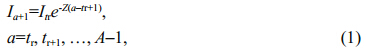
To make the results more estimable, we assume the values of Z are constant in the first nyears(e.g. the 1st–4th years when n is 4), and the value of Z for the first nyears is estimated using multiple cohorts CPUE data in this period. Then the value of Z for the second subsequent n years(the 2nd–5th years)is estimated and so on. Thus, Eq.1 can be rewritten as

Because multiple cohorts and multiple year data are used in one band and multiple band s need to be considered simultaneously when estimating Zx, the corresponding objective function used to estimate the time-based Z is
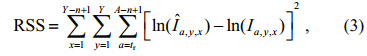
 a, y, x is the expected, Ia, y, x. The time-based Zs can be obtained by optimizing Eq.3.
2.2 Simulation scenarios
a, y, x is the expected, Ia, y, x. The time-based Zs can be obtained by optimizing Eq.3.
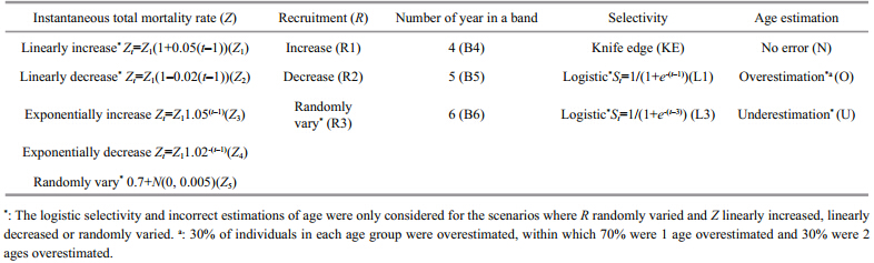
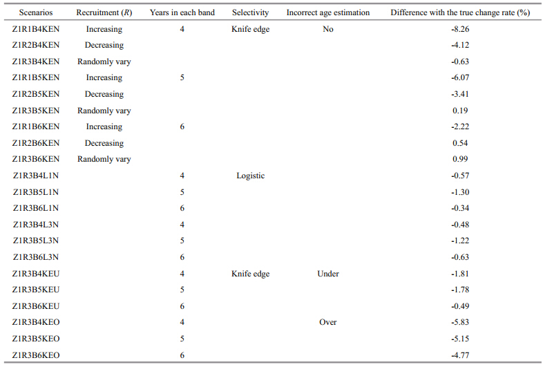
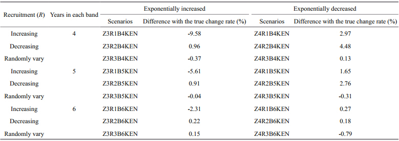
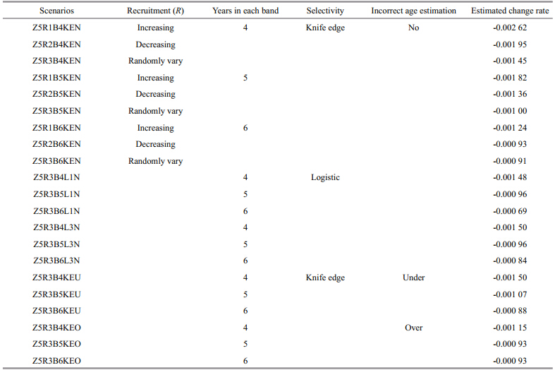
2.2 Simulation scenariosA total of 81 scenarios is developed to investigate the reliability of the method(Table 1). In all these scenarios, tr=1, A=8, and Y=20 are assumed, and the observation error of Iin data simulation is lognormally distributed with ln I– N(u, σ2), where σ=0.25, and CV is about 0.25. Five scenarios are considered based on the assumption of true Z, including linearly increasing, linearly decreasing, exponentially increasing, exponentially decreasing, and randomly varying(where change rate is zero). Three scenarios of Rvariation are assumed, including increasing, decreasing, and randomly varying. The number of years in each band is assumed to equal 4, 5 and 6 years to examine the effects of different years of data in one band on the estimation of Z. Knife edge selectivity, logistic selectivity, consistent overestimation of age and underestimation of age are also included in the simulation analyses. These factors affect the observed catch data. By adding them to the catch equation or the process of age determination, we test the accuracy of the estimated Z. In the scenario of consistent overestimation of age, 30% of individuals in each age group are overestimated, within which 70% are overestimated by 1 age and 30% are overestimated by 2 ages. The same method is also applied to the scenario of consistent underestimation of age, but each age is underestimated instead of overestimated. The scenarios of incorrect age estimations assumed here are more extreme than the actual situation in the real fisheries, thus the scenarios developed here can show the effects of incorrect age on the estimated results clearly. The logistic selectivity and incorrect estimations of age are only considered for the scenarios where R randomly vary and Z linearly increase, linearly decrease or randomly vary(see Table 1 for details of the explanation and symbols used to represent each scenario). For simplicity, we use abbreviations to represent the combination of each scenario, for example, Z1R3B4L1N means linearly increasing Z, randomly varying R, 4 years in one band, logistic selectivity withS50%=1, and no incorrect age estimation(see Tables 2–5 for details of the scenarios). For each scenario, 500 simulation runs are conducted to derive the stable results. To examine the change rates of the estimated Z values, we calculate the percentage of relative change rate of the estimated Zfor the first 4 Z scenarios and compared the estimated change rate with zero(the true change rate)for the 5th Zscenario. We compute the relative estimate error(REE)to examine the uncertainty of estimated Z(Jiao et al., 2004), which reflects the magnitude of error and the direction of bias at the same time. There are n years in each band, within which the estimated result can be regarded as the value of Z in any year. Therefore, we compare the estimated time-based Z values from all the band s with the true Z values in 3 ways, i.e. the estimated Z value of each band is compared with the first value, the last value and the median value in the corresponding band . Then we obtain different REE values, i.e. REE1, REE2 and REE3, which represent the closeness of the true value with the first, the last, and the median values of Z from each band, and they are calculated as follow:

 |
In order to examine the practicability of the method, we apply this method to the Atlantic cod(Gadusmorhua)fishery in the eastern Newfoundl and and Labrador. Atlantic cod is a demersal gadoid species found on both sides of the North Atlantic. The stock in the eastern Newfoundl and and Labrador, also called as northern cod, is one of the important economic mainstays. The stock collapsed during late 1980s and early 1990s owing to overfishing and environmental changes(Hutchings and Myers, 1994; Drinkwater, 2005). It is estimated, at one extreme, that fishing removed annually more than 70% of Newfoundl and ’s northern cod available to be caught in the late 1980s and early 1990s(Baird et al., 1992; Hutchings and Myers, 1994), and six cod populations in the world had collapsed by 1993. Therefore, mortalities(including fishing mortality and natural mortality)have long been the focus of attention for fisheries scientists. Using the method developed in this study, we estimated the Zs and change trend of northern cod during 1983 and 1997(Lilly et al., 2001).
 |
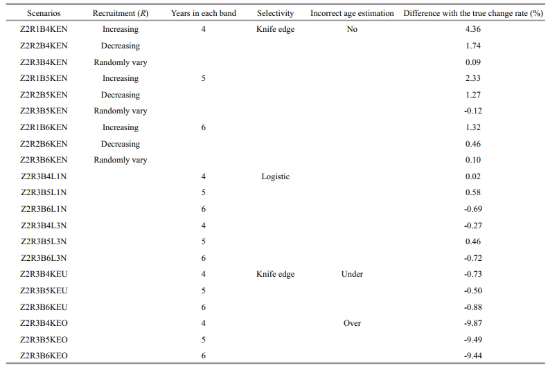 |
For all the 5 Z scenarios in this study, the trends of the estimated time-based Z values are consistent with the trends of true Z values. The estimated rates of change are not far from the true change rates(Tables 2–5 and Figs. 1–7). For the first 4 Z scenarios, the relative differences between the change rates of the estimated Z values and the true Z values are always smaller than 10%(Tables 2–4), and for the last Zscenario the absolute values of the change rate are close to zero(Table 5). Therefore, the change trends and change rates of the estimated Z values are not sensitive to the variation characteristics of the true Z values. Our research results show that both changes in recruitment and errors in ageing have limited effect on estimation of Z, and Z values are under-estimated when partial selectivity happened after recruitment, but the estimated change rates are not obviously affected by the variation of selectivity. The following sections will describe the influence from each factor with details.
 |
 |
When R is increasing, the REE1 and REE3 values of the estimated Zdecrease rapidly. However, the REEs are relatively stable for the scenarios of R decreasing and randomly varying(Fig. 1). REE2 values converge to about -6% for different years in one band in the scenario of Rincreasing, while for the other two Rscenarios REE2 values increase monotonically(Fig. 1).The values of REE are higher for the scenario of Rincreasing than those of Rdecreasing and randomly varying, which indicate increasing R is prone to result in larger estimated Zthan the other two R scenarios. The estimated Z values are impacted by different numbers of years in each band for different combinations of Z and R. Four years in one band result in relatively better results, i.e. REE is close to zero, for the scenario of Rincreasing. Conversely, when R is decreasing or randomly varying, all the REE values of 6 years in one band are closer to zero except for REE1, which are closer to zero for the scenario of 5 years in one band (Fig. 1). REE2 and REE3 of the estimated Z are smaller than zero for all the R scenarios, which mean values of Z are underestimated. However for REE1, we obtain different results for different R scenarios. Z values are overestimated for all the band scenarios when R is increasing. Scenarios of Z1R2B6KN, Z1R3B5KN and Z1R3B6KN give overestimated Z values, and other scenarios result in underestimated Z values(Fig. 1), indicating more years in one band are prone to give positive REE1 values of Z.
 |
|
Fig. 1 Trends of estimated and true values of instantaneous rate of total mortality(Z) and relative estimate error(REE, %)of estimated Z for different recruitment( R) and band scenarios when Z linearly increased The first row shows the estimated Z and the true Z; rows from the 2nd to the last shows the REE1, REE2 and REE3 . Bold solid line: true Z; diamond: 4 years in one band ; square: 5 years in one band ; and triangle: 6 years in one band. |
Figure 2 shows similar change trends of REE for different R scenarios, and we obtain relatively smaller absolute REE when Z and R share the same change trend(Fig. 2). Five years in one band give the smallest absolute REE1 values for all the R scenarios. However, the smallest absolute REE3 values appear in the scenario of 6 years in one band . The REE2 of different band scenarios in each Rscenario cluster, indicating similar estimated Z values are obtained(Fig. 2). REE2 values and REE3 values of Z are larger than zero, but for REE1 values, this depend on the R and band scenarios. When R is increasing, 4 and 5 years in one band resulted in overestimated Z values, but when Ris decreasing or randomly varying only 4 years in one band give overestimated Z values(Fig. 2).
 |
|
Fig. 2 Trends of estimated and true values of instantaneous rate of total mortality(Z) and relative estimate error(REE, %)of estimated Z for different recruitment( R) and band scenarios when Z linearly decreased See Fig. 1 for other explanation on rows and legends. |
The REE values decrease rapidly only when Z and R have the same change trend, and the REE values change faster when there are fewer years in one band . However, the REE values almost remain constant for other combinations of Z and R(Fig. 3). REE2 values and REE3 values of the estimated Z are smaller than zero for all the R and band scenarios, while REE1 values can be either higher or lower than zero. When R is increasing, the REE1 values are larger than zero except for the last 11 years in the scenario Z3R1B4KN. For the scenarios of Rdecreasing and randomly varying, only the REE1 s estimated from Z3R2B4KN, Z3R2B5KN, and Z3R3B4KN are smaller than zero. In the scenario of Rincreasing, 4 years in one band resulted in relatively smaller absolute REE1 values and REE2 values, and 6 years in one band give smaller absolute REE3 values. When Rare decreasing and randomly varying, the REE2 values and REE3 values approach to zero with the increase of the number of years in one band, but the smallest absolute REE1 values of the estimated Z, just like those in Figs.1 and 2, appeared in the scenario of 5 years in one band .
 |
|
Fig. 3 Trends of estimated and true values of instantaneous rate of total mortality(Z) and relative estimate error(REE, %)of estimated Z for different recruitment( R) and band scenarios when Zexponentially increased See Fig. 1 for other explanation on rows and legends. |
Like the scenario of Z linearly decreasing, REE values also show similar change trends with time for different Z scenarios, and the relatively better results appear when Z and R share the same change trend. The estimated Z values are relatively better compared with other Z scenarios since the absolute REE values are small and the REE values for different band scenarios are close, especially the REE2 values in scenarios of Z4R2, in which 3 band scenarios are tightly clustered(Fig. 4). The REE2 values and REE3 values of the estimated Z are larger than zero for all the R and band scenarios. However, the REE1 values of the estimated Zare larger than zero only in the scenarios of Z4R1B4KN, Z4R1B5KN, Z4R2B4KN, and Z4R3B4KN, indicating fewer years in one band are prone to give larger REE1 values of Z. Additionally, 5 years in one band give the smallest absolute REE1 values for all the R scenarios. For REE2 values and REE3 values, the smallest absolute values appeared in the scenarios of 6 years in one band .
 |
|
Fig. 4 Trends of estimated and true values of instantaneous rate of total mortality(Z) and relative estimate error(REE, %)of estimated Z for different recruitment( R) and band scenarios when Zexponentially decreased See Fig. 1 for other explanation on rows and legends. |
When the true Z is varying randomly, the change trends of the estimated time-based Zcan reflect the trends of true Zsince the change rates of the estimated Z are close to zero(Table 5), but the variations of the estimated Z values became smooth(Fig. 5). When Z is varying randomly, the REE values of the estimated Zalso randomly change. The errors of the estimated Zfrom different R scenarios are almost the same, and are higher than those when Z is increasing or decreasing over time. The REE3 values of the estimated Z are smaller than REE1 values and REE2 values for all the R scenarios(Fig. 5).
 |
|
Fig. 5 Trends of estimated and true values of instantaneous rate of total mortality(Z) and relative estimate error(REE, %)of estimated Z for different recruitment( R) and band scenarios when Z randomly varied See Fig. 1 for other explanation on rows and legends. |
For all the scenarios of 4, 5 and 6 years in one band, the values of REE2 and REE3 are always negative when Z is increasing, whereas when Z is decreasing we obtaine the opposite results((Figs. 1–4)). The REE1 values would be different depending on how many years are included in the band, and most of the Z values estimated from the scenario of 5 years in one band are close to the true values ((Figs. 1–4)). REE values from scenarios of Z exponentially increasing or decreasing are more stable than those from Zlinearly changing and randomly varying. When Z is increasing it is prone to be underestimated, and conversely when Z is decreasing it will be overestimated. Additionally, for each Zscenario the smallest and largest estimated Z values appeared in the scenarios of R decreasing and R increasing, respectively (Figs. 1–5). 3.8 Effects of partial selectivity and incorrect age determination
When partial selection happen after recruitment, Zvalues are underestimated, and the absolute REE values of the estimated Z are large for the scenarios of Z linearly increasing and randomly varying, meanwhile for the scenario of Z linearly decreasing the absolute REE values are relatively small(Fig. 6). When selectivity affected older ages(S50%increased from 1 to 3), the absolute REE values increase a lot, i.e. Z values are greatly underestimated(Fig. 6). However, the estimated change rates are not affected by the variation of selectivity. Incorrect age estimation can distort the estimate of utilized population(Ricker, 1971). The results show that both overestimation and underestimation of age can affect the estimates of Z. Simulation results indicate that underestimation of age result in overestimated Z, and overestimation of age result in underestimated Z(Fig. 7). When Z is linearly decreasing, the absolute values of the estimated REE are smaller than those when Z is linearly increasing or randomly varying(Fig. 7).
 |
|
Fig. 6 Relative estimate error(REE, %)of the estimated instantaneous rate of total mortality(Z)for different Z scenarios when recruitment randomly varied and selectivity followed logistic curve a: S50%=1; b:S50%=3. See the last columns of Figs.1, 2, and 5 for the results when selectivity follows knife edge curve. See Fig. 1 for other explanation on rows and legends. |
 |
|
Fig. 7 Relative estimate error(REE, %)of the estimated instantaneous rate of total mortality(Z)for different Z scenarios and recruitment randomly varied when(a): ages were underestimated, and (b): ages were overestimated See the last columns of Figs.1, 2, and 5 for the results without incorrect age estimation. See Fig. 1 for other explanation on rows and legends. |
The estimated Z of the Atlantic cod can be divided into 4 stages from 1983 to 1997(Fig. 8). Z slowly decreased from 1983 to 1987, and then increased rapidly in the next 4 years, i.e. from 1988 to 1991. During 1992 to 1994, Zdeclined rapidly, and followed by stable fluctuation. The number of years in each band (4, 5 and 6 years)do not give great impact on the estimated Zs the 1st, 3rd and the 4th stages(Fig. 8). However, the estimated Z values in the 2nd stage are greatly impacted by the number of year in the band, and more years in each band make the estimated Zvalue increased faster(Fig. 8). For all the scenarios of band, the largest value of Zappeared in 1991, while the smallest value of Zappeared in 1987.
 |
| Fig. 8 The time-based Z of cod(Gadus morhua)fishery of eastern Newfoundl and and Labrador from 1983 to 1997 |
Our newly developed approach to estimate timebased Z and its change trend using multiple cohorts CPUE data result in viable estimates of Z, and reveal the trends of time-based Z in practice. The method result in similar change rates of the estimated Z values with those of the true Z values. However, as it makes the estimated results smooth, the approach will be less useful for estimating the values of time-based Zwhen they fluctuate greatly over time and with a short period.
Both patterns of Z and R variation can affect the estimate of single Z in a band, and the combined effects that come from Z and Rmade the results more complicated. For the same Rscenario, the change trends of REE are significantly different among different Z scenarios. In contrast, for different scenarios of Runder the same Zscenario, the REE values of the estimated Zshow similar trends in changes although the values show some differences with each other(Figs.1–5). Therefore, the variations of Zhave more effect than that of Ron the estimate of the single Z in a band .
In this study, we considered scenarios of 4, 5, and 6 years in each band, and compared the estimated Zvalues with the true values of Z. The estimated Zvalues are close to the true Z values when appropriate nis determined, and the REE values of the estimated Z fluctuate around zero. Therefore, we cannot say whether fewer years or more years in the band are better. Fewer years means fewer data can be used in a band, and will make the estimated Z greatly fluctuate because of the r and om variation of the data, which decreases the credibility of the results. On the other side, more years in the band will lead to smoother estimated Z over time, which may not reflect the actual variation of Z. Because the most appropriate number of years considered in each band can be different given the effects of different factors(like Z and Rin this research), it is better to conduct simulation analyses before making a decision.
Selectivity and age determination are two important factors that can influence the stock assessment results in age-structure models. This is also true of the estimate of Zusing the approach developed here. Selectivity is a reflection of susceptibility to fishing gear. Knife edge selectivity means all the individuals of different ages are permitted to fish together at the start of the same year(Ricker, 1971). In this situation, Z values are estimated without the effects of protracted recruitment, and relatively better results will be obtained. However, fish grow differently and fishing gear is selective; therefore, the change of CPUE over time should not be due to the effects of Zalone, but also due to protracted recruitment caused by the selectivity patterns(King, 2007). Meanwhile, ages are sometimes estimated with error; if ages are overestimated or underestimated, Z will be under or overestimated by a catch curve. Although the estimated values of Zcan be impacted by the errors of selectivity and age estimation, our simulation results show that the approach is robust to estimate the change trends of time-based Z in spite of the impacts of these two kinds of errors(Figs.6, 7). Additionally, migration is also another source of error. If fishes migrate out of the fishing area, the measured decrease in CPUE should be due to the combined effects of Z and migration.
Besides above error sources, another error that may affect the performance of the developed method comes from the CPUE itself. CPUE is the most used index to represents the absolute abundance. Because of easy access, CPUE from many commercial and recreational fisheries is used in the assessment of fish populations, with strict proportionality between CPUE and abundance frequently assumed. However, it is reported that CPUE may not accurately reflect changes in abundance(Harley et al., 2001). The “hyperstability”, i.e. CPUE remaining high while abundance declines, usually exists(Hilborn and Walters, 1992), which may lead to underestimation of Z. The “hyperstability” is mainly affected by the spatial distribution of fish and the allocation of fishing effort. Therefore, to better underst and the relationship between CPUE and abundance, it is important to determine the extent to which fisher’s ability to locate the areas of greatest fish abundance interacts with habitat selection in fish(Harley et al., 2001). The collapse of Atlantic Cod has been discussed as one of the hottest topics in the world. Although several studies suggest a potential role for unfavorable climatic conditions(Rose et al., 2000; Rose, 2004; Halliday and Pinhorn, 2009), people agreed that overfishing is the primary factor that responsible for the decline of cod resource(Hutchings and Myers, 1994; Hutchings and Ferguson, 2000; Worcester et al., 2009). The abundance of the Atlantic Cod greatly decreased during the late 1980s and early 1990s. From 1982 to 1990 catches were above 200 000 t but declined to 172 000 t in 1991 before imposition of the moratorium on commercial fishing in 1992(Shelton et al., 1996). Correspondingly, our estimated Z increased rapidly during 1989 and 1991, and decreased after 1992, which proved our results are consistent with the variation of fishing intensity and abundance that mentioned in previous reports. During the moratorium, the fishing was absent, which means Zwas equal to M, thus the high total Zestimated during moratorium period indicated the possible high Mof this fishery instead of 0.2, which is commonly assumed. However, it must be pointed that the phenomenon of “hyperstability” may also exist in the Atlantic cod fishery. The collapse of the Atlantic cod fishery in Newfoundl and may be influenced by “hyperstability”, since cod aggregated in groups, but CPUE remained high, which covered the fact of decrease of abundance. Additionally, the effects of “hyperstability” were not analyzed in our simulation studies. Therefore, the CPUE of the Atlantic cod fishery may be biased, and we might underestimate Zs.
The death condition is very important to the analyses of fish population dynamics, the forecast of abundance and catch, and management of fisheries resources, so Z is one of the important parameters in fisheries science, and the estimation of Z is necessary and crucial. The method described in this paper can be used to estimate the time-based Z without complicated statistical catch-at-age analysis, and it is competent to estimate the change trends and change rates of the time varying true Z. Usually, Zcannot be accurately estimated each year because of the data quality and uncertainty factors(like selectivity and age determination mentioned above), therefore only a few estimated Z values can be treated as acceptable. In this case, it is valuable to know the change trend or the change rate of Z, which can estimate the variation of Z, and then judge the history of population dynamics and predict the probability of population variation. Usually, fishery researchers pay more attention to the variations of instantaneous fishing mortality rate(F)or Mbecause they can reflect the changes of fishing behavior or environmental factors, etc. Fhas direct relationship with catch, which is the most concern of fishermen and managers. M is included in all mathematical models of fish stock dynamics with the exception of simple surplus production models(Vetter, 1988). Thus, both of the two kinds of mortalities are important to fisheries research. However, both of them are not easy to accurately estimate, especially M, which is associated with biological and abiotic factors. Therefore, some researchers tried to estimate Mthrough Z- F. In such cases, the accurate estimate of time-based Z is particularly important. In addition, the estimated change rates of time-based Z from this method can be used as a prior study for other complicated methods, such as Bayesian theorem, to carry out in-depth studies on For M. We suggest that this method be considered when trend of Z is of concern for a fishery or complementary analysis on Z, F and /or M is needed. 5 CONCLUSION
The estimate of time-based Z is one of the important works in fisheries research, whose accurate estimate will greatly improve the results of stock assessment. In this research, we propose a catch curve-based method to estimate time-based Z, which can quickly estimate the values of Zusing multiple years’ CPUE data. The “b and ” considered in this method make the estimate of time-based Zmore accurate than traditional methods, and the most appropriate number of years considered in each band can be different given the effects of different factors, it is better to do simulation analyses before making a decision. However, the band method also smooth the values of the estimated time-based Z, and the values of Zmay be affected by many factors, like recruitment, selectivity, and errors of age determination, etc. In such situation, the approach is still competent to estimate the change trend or the change rate of Z, which can tell us the characteristics of variation of Z, and help us to judge the status of resources and then adjust the management strategies. 6 ACKNOWLEDGEMENT
We thank Dr. Roy Kirkpatrick, Yan Li, Man Tang and Matt Vincent for their valuable comments on an earlier draft.
| Baird J W, Bishop C A, Brodie W B, Murphy E F. 1992. An assessment of the cod stock in NAFO divisions 2J3KL.NAFO Scientific Council Research Document 92/18. |
| Beverton R J H, Holt S J. 1956. A review of methods for estimating mortality rates in exploited fish populations with special reference to sources of bias in catch sampling.Rapp. P.-V. Réun. CIEM, 140 : 67-83. |
| Butler S A. 1982. Estimation of fish mortality. Transactions of the American Fisheries Society, 111 : 535-537. |
| Chapman D G, Robson D S. 1960. The analysis of a catch curve. Biometrics, 16 : 354-368. |
| Deriso R B, Maunder M N, Pearson W H. 2008. Incorporating covariates into fisheries stock assessment models with application to Pacific herring of Prince William Sound,Alaska. Ecol ogical Appl ication, 18 : 1 270-1 286. |
| Drinkwater K F. 2005. The response of Atlantic cod (Gadus morhua) to future climate change. ICES Journal of Mar ine Sci ence, 62 : 1 327-1 337. |
| FAO. 2003. Fish Stock Assessment Manual. FAO Fisheries technical paper, Rome. p.393. |
| Fay G, Punt A E, Smith A D M. 2011. Impacts of spatial uncertainty on performance of age structure-based harvest strategies for blue eye trevalla (Hyperoglyphe antarctica). |
| Fish eries Res earch, 110 : 391-407. |
| Gaertner D. 2010. Estimates of historic changes in total mortality and selectivity for Eastern Atlantic skipjack (Katsuwonus pelamis) from length composition data.Aqual ic Living Resour ce, 23 : 3-11. |
| Haddon M. 2001. Modelling and Quantitative Methods in Fisheries. Chapman and Hall, New York. 405p. |
| Harley S J, Myers R A, Dunn A. 2001. Is catch-per-unit-effort proportional to abundance? Canadian Journal of Fisheries and Aquatic Sciences, 58 : 1 760-1 772. |
| Hilborn R, Walters C J. 1992. Quantitative Fisheries Stock Assessment: Choice, Dynamics and Uncertainty. Chapman and Hall, New York. 569p. |
| Hoenig J M. 1983. Empirical use of longevity data to estimate mortality rates. U. S. Fish ery Bull etin, 8 2 : 898-903. |
| Hutchings J A, Ferguson M. 2000. Temporal changes in harvesting dynamics of Canadian inshore fisheries for northern Atlantic Cod, Gadus morhua. Can adian J ournal of Fish eries and Aquat ic Sci ence, 57 : 805-814. |
| Hutchings J A, Myers R A. 1994. What can be learned from the collapse of a renewable resource? Atlantic cod, Gadus morhua, of Newfoundland and Labrador. Can adian J ournal of Fish eries and Aquat ic Sci ence, 51 : 2 126-2 146. |
| Jensen A L. 1996. Ratio estimation of mortality using catch curves. Fish eries Re s earch, 27 : 61-67. |
| Jiao Y, Chen Y, Schneider D, Wroblewski J. 2004. A simulation study of impacts of error structure on modeling stockrecruitment data using generalized linear models.Can adian J ournal of Fish eries and Aquat ic Sci ence, 61 : 122-133. |
| Jiao Y, Smith E P, O'Reilly R, Orth D J. 2012. Modelling nonstationary natural mortality in catch-at-agemodels. ICES Journal of Mar ine Sci ence, 69 : 105-118. |
| King M. 2007. Fisheries Biology, Assessment and Management.Second Edition. Blackwell, Malden. 400p. |
| Kizner Z I, Vasilyev D A. 1997. Instantaneous separable VPA (ISVPA). ICES Journal of Mar ine Sci ence, 54 : 399-411. |
| Lilly G R, Shelton P A, Brattey J, Cadigan N G, Healey B P,Murphy E F, Stansbury D E. 2001. An assessment of the cod stock in NAFO Divisions 2J+3KL. DFO Canadian Science Advisory Secretariat Research Document 2001/044. 148p. |
| Lorenzen K. 2005. Population dynamics and potential of fisheries stock enhancement: practical theory for assessment and policy analysis. Philosophical Transactions of the Royal Society B, 360 : 171-189. |
| NRC (National Research Council). 1998. Improving Methods for Fish Stock Assessment. National Academy Press,Washington DC.. |
| Quinn II T J, Deriso R B. 1999. Quantitative Fish Dynamics.Oxford University Press, New York. 542p. |
| Ricker W E. 1971. Derzhavin's biostatistical method of population analysis. J ournal of the Fisheries Research Board of Canada, 28 : 1 666-1 672. |
| Rijndorp A D, Daan N, Dekker W. 2006. Partial fishing mortality per fishing trip: a useful indicator of effective fishing effort in mixed demersal fisheries. ICES Journal of Mar ine Sci ence, 63 : 556-566. |
| Rose G A, deYoung B, Kulka D W, Goddard S V, Fletcher G L. 2000. Distribution shifts and overfishing the northern cod (Gadus morhua): a view from the ocean. Can adian J ournal of Fish eries and Aquat ic Sci ence, 57 : 644-664. |
| Rose G A. 2004. Reconciling overfishing and climate change with stock dynamics of Atlantic cod (Gadus morhua) over 500 years. Can adian J ournal of Fish eries and Aquat ic Sci ence, 61 : 1 553-1 557. |
| Schnute J T, Haigh R. 2007. Compositional analysis of catch curve data, with an application to Sebastes maliger. ICES J ournal of Mar ine Sci ence, 64 : 218-233. |
| Shelton P A, Stansbury D E, Murphy E F, Lilly G R, Brattey J. 1996. An assessment of the cod stock in NAFO Divisions 2J+3KL. DFO Atlantic Fisheries Research Document 96/80. |
| Thorson J T, Prager M D. 2011. Better catch curves: incorporating age-specific natural mortality and logistic selectivity. Transactions of the American Fisheries Society, 140 : 356-366. |
| Thorson J T, Simpfendorfer C A. 2009. Gear selectivity and sample size effects on growth curve selection in shark age and growth studies. Fish eries Res earch, 98 : 75-84. |
| Vetter E F. 1988. Estimation of natural mortality in fish stock: a review. Fish ery Bull etin, 86 : 25-43. |
| Wang Y B, Liu Q. 2006. Estimation of natural mortality using statistical analysis of fisheries catch-at-age data. Fish eries Res earch, 78 : 342-351. |
| Wayte S E, Klaer N L. 2010. An effective harvest strategy using improved catch curves. Fish eries Res earch, 106 : 310-320. |
| Worcester T, Brattey J, Chouinard G A, Clark D, Clark K J,Deault J, Fowler M, Frechet A, Gauthier J, Healey B,Maddock Parsons D, Mohn R, Morgan M J, Murhpy E F,Schwab P, Swain D P, Treble M. 2009.Status of AtlanticCod (Gadus morhua) in 2009. DFO Can. Sci. Advis. Sec.Res. Doc. 2009/027. v+112p. |
| Pope J G, Shepherd J G. 1982. A simple method for the consistent interpretation of catch-at-age data. Journal du Conseil / Conseil Permanent International pour l'Exploration de la Mer, 40 : 176-184. |
| Halliday R G, Pinhorn A T. 2009. The roles of fishing and environmental change in the decline of Northwest Atlantic groundfish populations in the early 1990's. Fish eries Res earch, 97 : 163-182. |