 2015, Vol. 33
Shanghai University
Article Information
- WEN Lijuan (文莉娟), NAGABHATLA Nidhi, ZHAO Lin (赵林), LI Zhaoguo (李照国), CHEN Shiqiang (陈世强)
- Impacts of salinity parameterizations on temperature simulation over and in a hypersaline lake
- Chinese Journal of Oceanology and Limnology, 2015, 33(3): 790-801
- http://dx.doi.org/10.1007/s00343-015-4153-3
Article History
- Received Jul. 7, 2014;
- accepted in principle Aug. 18, 2014;
- accepted for publication Oct. 8, 2014


2 Laboratory of Arid Climatic Changing and Reducing Disaster of Gansu Province, Cold and Arid Regions Environmental and Engineering Research Institute, Chinese Academy of Sciences, Lanzhou 730000, China;
3 Institut für Umweltplanung (IUP), Gottfried Wilhelm Leibniz Universität, Hannover 30419, Germany;
4 Asia-Pacific Economic Cooperation (APEC) Climate Center, Busan, 612020, Republic of Korea
Lakes have a considerable local impact on weather,climate, and hydrologic cycles. Lake-effect snow can affect transportation,commerce, and public safety of local communities. For example,an October 1984 snowstorm enhanced by the Great Salt Lake(GSL)effect produced nearly 70 cm deep snow within two days(Carpenter,1993),causing a million dollars in property damage. Accurate prediction of snowstorms is still one of the major forecast challenges in the area. It has been shown that lake surface skin temperature(LSST)can be related to the development of snowstorms from the GSL effect(Carpenter,1993; Steenburgh et al., 2000; Onton and Steenburgh, 2001; Crosman and Horel, 2009). LSST and its related nearsurface air temperature(NSAT) and lake temperature(LT)below the water surface significantly influence the atmospheric boundary layer,energy budget,local weather and climate(Bonan,1995; Lofgren,1997; Krinner,2003; Long et al., 2007; Mishra et al., 2011). Also affected are lake ecosystems,dissolved gas concentrations,biological productivity, and phenology(Magnuson and Bowser, 1990; McDonald et al., 1996; Crump et al., 2003; Mooij et al., 2008). Consequently,improvement in the accuracy of temperature simulation over and in the lake is important.
The GSL is hypersaline,with salinity 6%–28% in its south part and 16%–29% in its north part(Stephens,1990). Given that average salinity of seawater is around 3.5%,the GSL is much saltier. The salinity effect on surface evaporation has been studied(Carpenter,1993; Steenburgh and Onton, 2001). GSL saline composition can reduce moisture fluxes and result in a 17% reduction of snowfall compared with a freshwater body,as shown by Onton and Steenburgh(2001). In their study,salinity was parameterized to reduce water flux transport to the atmosphere by 10%. However,such a reduction in rate is not constant,as it varies with surface temperature and near-surface pressure. Apart from the impact on surface evaporation,salinity alters the heat capacity,thermal conductivity, and freezing point of lake water(UNESCO,1983; Wen and Jin, 2010a,b). All these parameters can influence temperature over and in the lake,but only some of them have been included in lake schemes for modeling saline lakes(Oroud,1995; Ali et al., 2001). Even in most numerical models in which there is no LT variable,LSST of saline lakes is simply replaced by forcing sea surface temperature as a freshwater lake or salinity effects are not considered in its simulation.
The twin objectives of the study were:(a)to parameterize salinity effects on water properties in a lake scheme to improve temperature simulation over and in the lake; and (b)to improve underst and ing of salinity effects on various water properties and their effects on temperature simulation. In this paper,we use the GSL study area with its available observation data for assessing model performance and its parameterizations of salinity effects on water properties. We show results from the simulations with and without the inclusion of salinity effects and from sensitivity experiments that tested those effects on water properties. 2 STUDY AREA AND DATA 2.1 GSL and its salinity
The GSL was separated into southern(Gilbert Bay) and northern(Gunnison Bay)parts by an east-west solid-fill railroad causeway,which has limited water mixing(Fig. 1). The southern part receives most of the inflow and thus becomes less salty than the northern part. The GSL is a terminal lake so its salinity variation is controlled by precipitation and evaporation over the entire basin. The United States Geological Survey(USGS)measures salinity periodically at intervals of 2 to 4 weeks. Based on measurements over the last 10 years,GSL salinity varies about 14.1% in Gilbert Bay and about 27.1% in Gunnison Bay. The lake has average depth 5 m. Diaz et al.(2009)indicated that measured salinity at depth 0.2 m was similar to that at 3 m. Therefore,in our simulation design,salinity was set to 14.1% for the south and 27.1% for the north,for the entire water column.
 |
| Fig. 1 Map of simulated domain including terrain height(m)(blue shading)of GSL area,the GSL(irregular black polygon),east-west solid-fill railroad causeway(bold red line), and observation stations(red left triangle,Gunnison Isl and ; red right triangle,Hat Isl and )
There were 40 lake grid points in model domain. |
Observed station temperature data to evaluate the model included daily NSAT and LT recorded at Hat(41.1°N,112.6°W) and Gunnison(41.3°N,112.9°W)isl and s,obtained from the MesoWest Project(Horel et al., 2002). NSAT is measured about 12 m above current lake level and LT in about 0.9 m of water,about 0.15 m above the lake floor. LSST used for model evaluation was from Moderate Resolution Imaging Spectroradiometer(MODIS)product data(MOD11C2,Version 005),from the National Aeronautics and Space Administration(NASA)L and Processes Distributed Active Archive Center. The MODIS product provides global 8-day composited and averaged daytime and nighttime l and surface temperature on 0.05-degree latitude/longitude grids. 3 MODEL AND SALINITY PARAMETERIZATIONS3.1 Model
We used the Weather Research and Forecasting model version 3.0 coupled with Community L and Model version 3.5(WRF-CLM)(Subin et al., 2011). The WRF model is one of the most widely used and advanced regional atmospheric models,involving a nonhydrostatic computational fluid dynamics core and several physical parameterizations for unresolved atmospheric processes(Skamarock and Klemp, 2008). Calculated low-level variables(wind,temperature,humidity,radiation and pressure)were transferred to force the l and surface model CLM.
The CLM model(Oleson et al., 2004)treats the l and surface as five primary subgrid l and -cover types(glacier,lake,wetl and ,urban,vegetated)on each grid cell. The calculated energy,water, and momentum fluxes in each grid can be passed to the atmospheric model WRF.
For the lake subgrid l and cover in the CLM model,lake processes and lake-atmosphere interactions are dynamically simulated using a 1-D mass and energy balance lake scheme with 10 lake water layers(Oleson et al., 2004). This lake scheme was developed based on previous studies(Henderson-Sellers,1985; Hostetler and Bartlein, 1990; Hostetler et al., 1993; Hostetler et al., 1994; Bonan,1995; Zeng et al., 2002). In the CLM model,calculation of surface fluxes of lake similar to that of non-vegetated surfaces. LSST can be computed using the surface fluxes at the same time. With surface net energy flux as the top boundary(Oleson et al., 2004),thermal mixing between simulated lake layers is mainly under the control of wind-driven eddies,convection, and molecular diffusion(Hostetler and Bartlein, 1990; Zeng et al., 2002; Oleson et al., 2004). The Crank-Nicholson thermal diffusion solution is used to calculate lake temperature of each layer(Oleson et al., 2004). 3.2 Model settings
The center of the simulated domain is 41.0°N,112.5°W. The horizontal dimension is 1 000 km× 1 000 km with 10-km grid spacing. The GSL occupies 40 grid points and the whole simulated domain is about 100×100 grid points. With the higher resolution near the surface,there were 31 vertical layers in the simulation. Initial and lateral boundary conditions were from North American Regional Reanalysis(NARR; horizontal resolution 32 km×32 km)data(Mesinger et al., 2006),updated every 3 hours. Lake depth was set to the average GSL depth(5 m)in the model. In total,there were 10 lake water layers,at 0.05,0.15,0.3,0.6,0.9,1.4,2,2.7,3.5, and 4.5 m below the lake surface. The final choice of physical options was made based on a number of sensitivity tests,including Morrison double-moment(Morrison et al., 2005),Dudhia scheme(Dudhia,1989),KainFritsch scheme(Kain,2004),Rapid Radiative Transfer Model(RRTM)scheme(Mlawer et al., 1997),plus CLM3.5(Oleson et al., 2008) and Yonsei University(YSU)scheme(Noh et al., 2003). The model was run from September 3,2001 to September 30,2002,during which sea surface temperature had average conditions. Simulations for the first month were treated as spin-up, and discarded. The model output data hourly,including multi-layer wind,humidity,pressure,air temperature,soil moisture,soil temperature,lake temperature,surface temperature,radiation,latent heat flux,sensible heat flux,precipitation, and others. 3.3 Salinity parameterizations
The high salinity of the GSL can affect lake water properties. Owing to this salinity,the GSL almost never freezes,except at freshwater inlets(Steenburgh et al., 2000). However,the original version of the lake scheme included in the WRF-CLM model only h and les freshwater lakes. To study the GSL,the salinity effect on water properties should be parameterized in the model. We present in the following sections parameterizations of salinity effects on lake water properties(heat capacity,thermal conductivity,freezing point and saturated vapor pressure)in the WRF-CLM model. 3.3.1 Salinity parameterization of heat capacity
3 The heat capacity of the saltwater is related to the proportions of substances(water and salt)that it contains. Water has the highest heat capacity,save for liquid ammonia. After dissolving salt into water,the water mass portion is reduced. The higher the salinity,the lower the heat capacity of saltwater,without considering effects of pressure and temperature. The fitted linear equation(Sun et al., 2008)for saline water heat capacity and salinity(s)at 20°C and 100°C can be written as
where cpsw and cpfware specific heat capacities ofsaline water and fresh water,respectively. The rate of decrease of heat capacity with salinity for the above two temperatures is the same,at 4.4 kJ/(kg∙K). Even at a high temperature of 180°C,the lapse rate is only slightly higher(4.6 kJ/(kg∙K)). Consequently,the rate of decrease in Eq.1 is introduced into the model to consider the heat capacity change of saltwater with salinity variation. cpfwwas approximated as 4.156 9 and 4.198 4 kJ/(kg∙K)at 20°C and 100°C,respectively(Sun et al., 2008). The heat capacity change of saltwater with temperature need not be considered in the model because the original specific heat capacity in the model is simply set to 4.188 kJ/(kg∙K),which is similar to the values used in Eq.1 at 20°C and 100°C. To be consistent with the original lake scheme in the WRF-CLM model,the following equation(Wen and Jin, 2010b)was applied in the lake scheme. 3.3.2 Salinity parameterization of thermal conductivity

Freshwater thermal conductivity λfwin the model was set to 0.6 W/(m∙K),which is that at 20°C. Water thermal conductivity decreases with increasing salinity. Thermal conductivity of a NaCl solution was used to replace that of GSL water in the model,because NaCl represents ~76% of dissolved salts in the lake(Dickson et al., 1965). Thermal conductivity of a NaCl solution(Yusufova et al., 1975; Ozbek and Phillips, 1980; Diguilio and Teja, 1992)was fit to the observations as
λsw and λfware the thermal conductivities of saltwater and freshwater,respectively, and Tis temperature(°C). Consistently with the original model,the change of λswwith temperature is not considered. Thus,the thermal conductivity accounting for salinity in the model(Wen and Jin, 2010b)was set to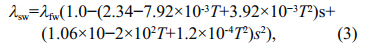

Solving Eq.4 using salinities of 13.6% and 25.2% gives λswof 0.583 and 0.571 W/(m∙K),respectively,which are close to the experimental values 0.583 and 0.577 W/(m∙K)for salinities of 13.6% and 25.2%(Ozbek and Phillips, 1980). Therefore,Eq.4 seems reasonable. 3.3.3 Salinity parameterization of freezing point
Fresh water freezes at 0 ℃. Adding salt to water remarkably decreases the freezing point. Water molecules in saltwater do not easily encounter one another because their interactions are interfered by surrounding salt particles. This makes it more difficult for saltwater to form ice and easier to melt once formed. A study by the National Snow and Ice Data Center(NSIDC)showed that the freezing point decreases by 0.28°C for every 0.5% increase in salinity(http://nsidc.org/cryosphere/seaice/characteristics/ brine_salinity.html). The equation
was used in the lake scheme of the WRF-CLM model(Wen and Jin, 2010a,b),in which Tfis the freezing point(°C). Salt components of the GSL are 75.91% NaCl,10.92 MgCl2,9.52% Na2SO4,3.16% KCl, and others(Dickson et al., 1965). Putting solutions with similar salt composition(77% NaCl,10% MgCl2,10%Na2SO4,3% KCl)in the refrigerator,ice begins to appear at -8.5°C and -15°C in solutions with 14.1% and 27.1% salinities,respectively. The calculated freezing points using Eq.5 are -7.9 and -15.0°C,respectively. Equation 5 seems to work reasonably. 3.3.4 Salinity parameterization of saturated vapor pressure
Saltwater evaporates more slowly than freshwater,because ions help to maintain water molecules in a liquid state. The high salinity(27.1%)in Gunnison Bay was found to reduce the saturated vapor pressure over the water surface by 20%–40%. Using Raoult’s law,the calculated ratio α of saturated vapor pressure over saltwater to that over freshwater was far from that observed in the GSL for high salinity,but the following equation(Low,1969),
appeared to work better than Raoult’s law for the GSL(Dickson et al., 1965; Steenburgh et al., 2000),in which,mis the salt molar concentration-molality: and γis the sodium-chloride activity coefficient. Therefore,Eq.6 was chosen for application in the salinity effect modeling study. However,γmust be provided for this application, and it varies with salinity and temperature. γis 0.82,0.68,0.70, and 0.87 at 25°C with molalities 0.05,0.50,2.00 and 5.00 mol/kg; these correspond to salinities by mass of approximately 0.3%,3%,10% and 23%. From 25°C to 50°C,γonly changes from 0.82 to 0.81 with molality 0.05 mol/kg, and from 0.87 to 0.89 with molality 5 mol/kg(Cohen and Paul, 1989). Variationof γdoes not change very significantly with normal temperature and salinity. To apply Eq.6 to the model,this variation was ignored and γwas set to 0.77,which is the average of various molalities at 25°C. The equation applied to the lake(Wen and Jin, 2010b)was changed to


The calculated αusing Eq.8 is 88% and 77% for salinities 14.1% and 27.1%. The observed αis about 80% with salinity 24.7%,between 5°C and 25°C(Dickson et al., 1965; Calder and Neal, 1984). The parameterization with Eq.8 appears reasonable.
In the original model,the 36 coefficients of eighthorder polynomial fits for saturated vapor pressure were only suitable for the 0 to 100°C range over water surface and -75 to 0°C over ice(Flatau et al., 1992). To match the extended freezing point,36 coefficients suitable for -85 to 70°C over water and -90 to 0°C over ice were also provided by Flatau et al.(1992) and were used in our study. Flatau et al.(1992)also gives 72 related coefficients and eighth-order polynomial fits. 3.4 Model experiments
Two experiments using WRF-CLM were performed to show the salinity effect on local climate simulation,as explained below:
1)FreshLake experiment. Without considering the salinity effect,the original WRF-CLM model was used for simulation. Model settings were as in Section 3.2;
2)SaltLake experiment. Similar to the FreshLake experiment,but with parameterizations of salinity effects.
To show the salinity effect on lake temperature induced by individual lake water property changes,four more sensitivity experiments were performed,as below:
1)Heat capacity experiment(HC). Similar to the SaltLake experiment but with heat capacity of freshwater ;
2)Thermal conductivity experiment(TC): similar to the SaltLake experiment but with thermal conductivity of freshwater ;
3)Freezing point experiment(FP): similar to the SaltLake experiment but with freezing point of freshwater ;
4)Saturated Vapor Pressure experiment(SVP): similar to the SaltLake experiment but with saturated vapor pressure over freshwater .4 RESULT 4.1 Simulated temperature over and in the GSL
Given that the results for Hat and Gunnison isl and s were similar,we mainly focused our analysis on the former,but still give some information on the latter. Simulated daily NSAT,LSST and LT at Hat Isl and are shown in Fig. 2a,b and c,respectively,in comparison with observed temperature.
 |
| Fig. 2 Observed and simulated daily temperature from FreshLake and SaltLake experiments |
Both FreshLake and SaltLake experiments captured very well the variations of the observed daily NSAT from October 1,2001 to September 30,2002(Fig. 2a). The two simulations were similar and close to observations for observed NSAT warmer than 0°C. However,the FreshLake simulation showed temporal short-term deviations relative to observations during the coldest event of winter. Observed daily NSAT was -8.1°C on January 30,2002. The simulated NSAT was -6°C in the SaltLake experiment,which was a small overestimation by 2°C. In the FreshLake experiment,the simulated NSAT was -17°C for the same day,which was a large underestimation by 9°C. Therefore,it appears that including the salinity effect in simulation can improve prediction of NSAT temperature in a cold event. Consideration of the salinity effect in the model: 1)clearly reduces the maximum daily negative bias of simulated NSAT,mainly improving the period with ice in the FreshLake experiment; 2)alters the median value of daily bias from -0.8 to -0.2°C(Fig. 3),mainly improving the icefree period in that experiment.
The FreshLake and SaltLake experiments simulated LSST well. Similar to NSAT simulation,the former experiment significantly underestimated LSST in the very cold event(Fig. 2b). The maximum negative difference between simulation and observation decreased from 15.8°C to 8.1°C for the FreshLake and SaltLake experiments,respectively(Fig. 3).
 |
| Fig. 3 Box plots with median,minimum/maximum, and 25th/75th percentiles of time series of daily temperature differences between observations and simulations,from SaltLake and FreshLake experiments |
As shown earlier in Fig. 2c,when observed LT was warmer than 0°C,both FreshLake and SaltLake experiments represented very well daily variations of LT,but both experiments showed quantitative underestimation of LT,which was particularly evident towards higher temperatures. Nevertheless,the underestimation in the SaltLake experiment was slightly less than that in the FreshLake experiment for the ice-free period. In winter,the simulated LT of FreshLake was nearly constant,showing a flat pattern at approximately 0°C,while the observed LT was less than 0°C. For the same period,the simulation performed much better in the SaltLake experiment,in which the simulated LT had fluctuations and magnitudes similar to the observed LT. There was signifi cant improvement in negative LT bias difference in the SaltLake experiment relative to the FreshLake experiment(Fig. 3). There was almost no bias(median difference near 0 ℃)in the SaltLake experiment.
As evident in Figs.2 and 3,the most typically used bias and root mean square errors(RMSE)for model evaluation(Bennett et al., 2013)also indicated that the SaltLake experiment had smaller errors(Table 1) and better simulation for both Hat and Gunnison isl and s. By including salinity parameterizations,the model was improved for more accurate temperature simulation in the saline lake.
 |
The simulated lake albedo(<0.2)at Hat Isl and was identical in both experiments when the freshwater lake thawed(Fig. 4). When the fresh water froze,there was ice(with much higher albedo than unfrozen water)in the lake in the FreshLake experiment,which increased lake albedo. With variation in temperature,albedo maximized at 0.6 and fluctuated with the appearance and disappearance of ice in the FreshLake experiment. In the SaltLake experiment with inclusion of salinity,winter albedo was generally less than 0.2,since the saline lake was free of ice. Because the GSL never completely freezes and ice only appears at the freshwater inlets,albedo simulated in the SaltLake experiment was considered more realistic. Apparently,salinity parameterizations in the model improved albedo simulations in the cold season and temperature simulations over and in the lake.
 |
| Fig. 4 Simulated daily albedo in FreshLake,SaltLake, and FP experiments |
Four parameters related to salinity were modified and contributed to temperature simulation improvement in the SaltLake experiment. To show the impact of each factor’s change on this improvement,four additional specific sensitivity experiments based on the SaltLake experiment were performed. 4.2.1 Impact of heat capacity change
To underst and the relationship between heat capacity and salinity and evaluate potential effects of altered heat capacity on local climate simulation,the HC experiment was conducted. The experimental design was almost the same as the SaltLake experiment,but with heat capacity set to the value of freshwater(4.188 kJ/(kg∙K)). However,the specific heat capacity calculated from Eq.2 for the 14.1% and 27.1% salinities of the southern and northern GSL were 3.57 and 3.00 kJ/(kg∙K)in the SaltLake experiment.
LSST simulated in the sensitivity experiments is shown,because NSAT and LT were found highly correlated with LSST. At Hat Isl and with 14.1%salinity,the average daily LSST difference between the HC and SaltLake experiments fluctuated with variation in daily temperature(Fig. 5a). Generally,the differences were less than 2°C. The average monthly LSST difference between the SaltLake and HC experiments was nearly positive from March through July at Hat Isl and (Fig. 5b)when the temperature was generally rising. Average monthly LSST in the SaltLake experiment was less than that in the HC experiment from October through January at Hat Isl and ,when the temperature was typically declining. The largest negative difference(-0.4°C)of monthly average LSST between the SaltLake and HC experiments was in December(Fig. 5b).
 |
| Fig. 5 Simulated daily and monthly LSST differences between SaltLake and HC experiments |
At Gunnison Isl and (figure not shown)with 27.1% salinity,the largest negative monthly LSST difference between the two experiments was about -0.8°C in December. Its absolute value was greater than that at Hat Isl and (-0.4°C). In addition,the magnitude of average LSST difference from October through January(March through July)at Gunnison Isl and ,with value -0.4°C(0.3°C),was also greater than that at Hat Isl and ,-0.2°C(0.2°C).
In general,setting a lower heat capacity in the SaltLake experiment resulted in greater temperature variation. LSST in the SaltLake experiment was higher(lower)than that in the HC experiment with temperature rise(decline). The higher the salinity,the greater the observed change. 4.2.2 Impact of thermal conductivity change
According to Eq.4,thermal conductivity in the model was 0.58 and 0.57 W/(m∙K)for the southern and northern GSL waters,with salinities 14.1% and 27.1%,respectively. The higher the salinity,the lower thermal conductivity of saltwater. To underst and the effect of thermal conductivity difference caused by salinity on local climate,the TC experiment was conducted. This was almost identical to the SaltLake experiment,but with modified thermal conductivity set to the value of freshwater(0.6 W/(m∙K)).
The difference in simulated mean LSST between the SaltLake and TC experiments was near zero(figure not shown). Therefore,it appears that the influence of thermal conductivity difference can be neglected. There are two reasons for this. First is that thermal conductivity change induced by salinity was small,only 0.02–0.03 W/(m∙K). Second is that thermal conductivity mostly affects molecular diffusion,whereas eddy diffusion and convection are more important in thermal mixing of the lake. 4.2.3 Impact of freezing point change
The freezing points of -7.9 and -15.0 ℃ calculated using Eq.5 with salinities 14.1% and 27.1%,respectively,were used in the GSL simulation,which makes GSL ice nearly unfreezable in winter. To see the impact of freezing point change,the FP experiment was conducted,with the freezing point set to 0 ℃ as in freshwater and other parameters kept identical to the SaltLake experiment.
The simulated average daily LSST in the FP experiment was the same as that in the SaltLake experiment when LSST was warmer than 0 ℃(Figs.2 and 6). During that period,change in freezing point had no impact on the simulation.
From mid November through mid March,when the daily minimum LSST in FP experiment was less than 0 ℃,monthly average LSST in the SaltLake experiment was warmer(~1 ℃)than that in the FP experiment at both Hat and Gunnison isl and s(Fig. 6b). The largest monthly difference was ~4.1 ℃ in February at Hat Isl and with 14.1% salinity, and 3.2°Cat Gunnison Isl and with 27.1% salinity. The largest daily difference between the two experiments was 14.5 ℃(12.2 ℃)during the coldest winter event at Hat(Gunnison)Isl and (Fig. 6a).
 |
| Fig. 6 Simulated daily and monthly LSST differences between SaltLake and FP experiments |
The LSST difference was mainly induced by different lake surface phases in the SaltLake and FP experiments for winter. When LSST was less than 0 ℃ and greater than the saltwater freezing point,the lake surface phase was ice in the FP experiment and water in the SaltLake experiment,respectively. The variable surface phases induced different heat capacities of the interface between lake and air. These were 2.12 kJ/(kg∙K)for ice in the FP experiment,3.57 kJ/(kg∙K)for water with 14.1% salinity, and 3.00 kJ/(kg∙K)for water with 27.1% salinity in the SaltLake experiment. Lake surface ice cause LSST to change more quickly than lake surface water under the same conditions with no ice.
Furthermore,the phase change can reduce energy loss in the SaltLake experiment for winter compared with that of the FP experiment. At Hat Isl and ,change of lake surface phase from water to ice increased average albedo from 0.1 in the SaltLake experiment to 0.4 in FP(Fig. 4)from mid November through mid March,with a corresponding reduction of average net solar radiation from 93 W/m2in SaltLake experiment to 67 W/m2in FP experiment. Average latent(sensible)heat flux decreased from 46(6)W/m2in the SaltLake experiment to 36(-3)W/m2in FP during the same period. In summary,energy loss of the SaltLake experiment for winter was generally less than that of the FP experiment. Thus,LSST in the FreshLake experiment dropped more significantly in winter with the appearance of ice induced by the high FP of freshwater. 4.2.4 Impact of saturated vapor pressure change
Saltwater is associated with slower evaporation than freshwater under the same meteorological conditions,because of a reduction in saturated vapor pressure over saltwater. To investigate the effect of saturated vapor pressure change caused by salinity,the SVP experiment was conducted by adopting the saturated water pressure over freshwater and leaving other options exactly the same as in the SaltLake experiment.
The average daily LSST in the SVP experiment was slightly lower than that in the SaltLake experiment throughout the year,with occasional exceptions(Fig. 7a). The difference was relatively stable in warm periods and was approximately between 0.5 ℃ and 1.5 ℃. However,in cold periods,the difference changed dramatically; the maximum change was as large as 7.5 ℃. There were also occasional negative daily differences in winter. The average monthly LSST in the SVP experiment was always lower than that of SaltLake throughout the year(Fig. 7b). The largest monthly difference was ~1.2 ℃(1.4 ℃)at Hat(Gunnison)Isl and with 14.1%(27.1%)salinity. Annual average LSST in the SVP experiment was ~0.6 ℃(1.1 ℃)colder than that in the SaltLake experiment with 14.1%(27.1%)salinity.
 |
| Fig. 7 Simulated daily and monthly LSST differences between SaltLake and SVP experiments |
The relatively low LSST in the SVP experiment is probably attributable to the decrease of saturated vapor pressure over the saline water surface,so the SVP experiment had greater latent heat flux and more energy loss from the lake surface. The simulated annually averaged latent heat flux in the SaltLake experiment at Hat Isl and with 14.1% salinity was ~3.7 W/m2less than that of the SVP experiment(~123 W/m2). The value in the SaltLake experiment was about 97.5% to that in the SVP experiment. The reduction of average latent heat flux also occurred at Gunnison Isl and (27.1% salinity),but with a larger reduction ratio(90.3%). 5 DISCUSSION
This study mainly focused on temperature over and in the Great Salt Lake. The area of the GSL,occupying 40 grids in the simulated domain,is less than 1% of the simulated domain that is about 100×100 grids. Simulated temperature(Fig. 2 and Table 1) and precipitation(figure not shown)in the SaltLake experiment were reasonable and similar to observations. Therefore,the 1 000×1 000 km simulated domain was used,although it is small compared with a typical regional climate simulation and the simulated results may be influenced by setting of the lateral boundary.
Simulations from September 3,2012 to August 31,2013 were performed. The modified WRF-CLM model was proven to have better simulation. The simulated results had some interannual variability compared with those from September 3,2001 to September 30,2002,but the salinity effect on temperature simulation was very similar.
The modified WRF-CLM model can reasonably simulate temperatures over and in the GSL,but there is still potential for improvement. First,the salinity was set to a fixed value for the northern and southern GSL in the simulated period,respectively. In reality,salinity is expected to have seasonal and interannual variations with changes in inflow,precipitation and evaporation,the appearance and melting of ice on the lake. Limited by this assumption,salt in the lake water must follow phase changes of that water in the model. Second,the difference between freezing point of GSL water and melting point of lake ice was not considered. Physically,the melting point of frozen saline lake ice should be similar to that of sea ice. Salt in sea ice will be rejected out with time. However,the ice never loses the salt instantaneously(Notz and Worster, 2008). Even for very thin sea ice with rapid development,it takes 24 h to reject out most of the salt. In slow-growing ice,it takes several days until the ice contains less salt. The melting point of sea ice is determined by bulk salinity,which is dependent on the solid fraction in ice and brine salinity. In new sea ice,the solid fraction is very low and bulk salinity approximates brine salinity(Notz and Worster, 2008). Bulk salinity at the interface of sea ice with solution is nearly the same as that of solution(Notz and Worster, 2008). The main body of the GSL never freezes. If there is occasionally a small amount of ice on the main GSL body,it is new ice surrounded by salt lake water, and will therefore disappear quickly. Thus in our case,the melting point of ice in the GSL does not have big difference with the freezing point of the GSL water. Therefore,in our modified model,we did not consider the difference between freezing point of GSL water and melting point of ice in the GSL. Third,the vertical gradient of salinity and salinity effect on density(Wen and Jin, 2010a,b; Naftz et al., 2011)were not considered in the simulation. A small vertical salinity gradient difference will affect mixing of the lake water. To test this,we must obtain a very accurate vertical salinity gradient. Fourth,lake depth was set to 5 m,whereas actual depth across the lake may differ,with a maximum ~10 m. In future studies,these limitations could be overcome by more observations and including more complex lake parameters at the expense of greater numerical resources.
Despite these simplifications in the modified WRFCLM,parameterizations of the salinity effect in a lake scheme clearly improved temperature simulation over and in the saline lake. A lake scheme with salinity parameterization can form a module of the CLM model for lake subgrid l and cover. Apart from the WRF-CLM,the CLM is widely used in the Community Earth System Model(CESM),Community Climate System Model(CCSM),Regional Climate Model system(RegCM), and other models. For similar cases,parameterizations of salinity effect from the present study could be applied to these models directly,or after code modifications. The lake scheme used herein has many similarities with the Hostetler lake scheme,which is also used as an offline lake model(Small et al., 2001; Perroud et al., 2009; Martynov et al., 2010)or coupled with a regional climate model,such as the Canadian Regional Climate Model(Martynov et al., 2012),for lake studies. The parameterization of salinity effect in the present study can also be useful in these models for similar applications. 6 CONCLUSION
In the present study,the salinity effect on lake water properties(heat capacity,thermal conductivity,freezing point, and saturated vapor pressure)was parameterized in the lake scheme of the WRF-CLM model. The modified WRF-CLM model was used to simulate temperature over and in the GSL from September 3,2001 to September 31,2002, and to study contributions of the salinity effect on lake water properties to temperature simulation with sensitivity experiments. Model simulation results show that the modified WRF-CLM model,which includes the salinity effect in its lake scheme,could more reasonably simulate temperature over and in the GSL. The modified model had superior accuracy compared to neglecting the salinity effect,particularly during very cold periods. The remarkable performance of the model simulation in the cold season is mainly attributable to consideration of the salinity effect on freezing point. This effect never allows the GSL to completely freeze,except at its freshwater inlets(Steenburgh et al., 2000). Another consequence is the change in lake surface phase from ice to water during the cold season,which reduces albedo. Hence,including salinity alters the energy balance of the lake surface in the model,thereby making it more realistic. The salinity effect on saturated vapor pressure can reduce latent heat flux and make the lake slightly warmer. A smaller heat capacity in the SaltLake experiment made lake temperature more prone to change. The salinity effect on thermal conductivity appears to be insignificant in the simulation of salt lakes. 7 ACKNOWLEDGEMENT
The first author thanks Dr. JIN Jiming at Utah State University to invite her as a visiting scholar in his laboratory to do part of the work. We also acknowledge support for using the computing resources at the Supercomputing Center of Cold and Arid Regions Environmental and Engineering Research Institute,Chinese Academy of Sciences.
| Ali H, Madramootoo C A, Gwad S A. 2001. Evaporation model of Lake Qaroun as influenced by lake salinity.Irrig. Drain., 50 (1): 9-17. |
| Bennett N D, Croke B F W, Guariso G, Guillaume J H A,Hamilton S H, Jakeman A J, Marsili-Libelli S, Newham L T H, Norton J P, Perrin C, Pierce S A, Robson B, Seppelt R, Voinov A A, Fath B D, Andreassian V. 2013.Characterising performance of environmental models.Environ. Modell. Softw, 40 : 1-20, http://dx.doi.org/10. 1016/j.envsoft.2012.09.011. |
| Bonan G B. 1995. Sensitivity of a GCM simulation to inclusion of inland water surfaces. J. Climate, 8 (11): 2 691-2 704. |
| Brock T D. 1975. Salinity and the ecology of dunaliella from Great Salt Lake. J. Gen. Microbiol., 89 : 285-292. |
| Calder I R, Neal C. 1984. Evaporation from Saline Lakes—a combination equation approach. Hydrol. Sciences J., 29 (1): 89-97. |
| Carpenter D M. 1993. The lake effect of the Great Salt Lake— overview and forecast problems. Weather Forecast, 8 (2): 181-193. |
| Cohen P. 1989. The ASME Handbook on Water Technology for Thermal Systems. American Society of Mechanical Engineers, New York. 1900p. |
| Crosman E T, Horel J D. 2009. MODIS-derived surface temperature of the Great Salt Lake. Remote Sens. Environ., 113 (1): 73-81. |
| Crump B C, Kling G W, Bahr M, Hobbie J E. 2003.Bacterioplankton community shifts in an arctic lake correlate with seasonal changes in organic matter source.Appl. Environ. Microb., 69 (4): 2 253-2 268, http://dx.doi. org/10.1128/Aem.69.4.2253-2268.2003. |
| Diaz X, Johnson W P, Naftz D L. 2009. Selenium mass balance in the Great Salt Lake, Utah. Sci. Total. Environ., 407 (7): 2 333-2 341. |
| Dickson D R, Yepson J H, Hales J V. 1965. Saturated vapor pressures over Great Salt Lake brine. J. Geophys. Res., 70 : 500-503. |
| Diguilio R M, Teja A S. 1992. Thermal conductivity of aqueous salt solutions at high temperatures and high concentrations.Ind. Eng. Chem. Res., 31 (4): 1 081-1 085. |
| Dudhia J. 1989. Numerical study of convection observed during the Winter Monsoon Experiment using a mesoscale two dimensional model. J. Atmos. Sci., 46 (20): 3 077-3 107. |
| Flatau P J, Walko R L, Cotton W R. 1992. Polynomial fits to saturation vapor-pressure. J. Appl. Meteorol., 31 (12): 1 507-1 513, http://dx.doi.org/10.1175/1520-0450(1992) 031<1507:Pftsvp>2.0.Co;2. |
| Henderson-Sellers B. 1985. New formulation of eddy diffusion thermocline models. Appl. Math. Model., 9 : 441-446. |
| Horel J, Splitt M, Dunn L, Pechmann J, White B, Ciliberti C,Lazarus S, Slemmer J, Zaff D, Burks J. 2002. Mesowest: cooperative mesonets in the western United States. B. Am.Meteorol. Soc., 83 (2): 211-225. |
| Hostetler S W, Bartlein P J. 1990. Simulation of lake evaporation with application to modeling lake level variations of Harney-Malheur Lake, Oregon. Water Resour. Res., 26 (10): 2 603-2 612. |
| Hostetler S W, Bates G T, Giorgi F. 1993. Interactive coupling of a lake thermal model with a regional climate model. J.Geophys. Res., 98 (D3): 5 045-5 057. |
| Hostetler S W, Giorgi F, Bates G T, Bartlein P J. 1994. Lakeatmosphere feedbacks associated with paleolakes Bonneville and Lahontan. Sci., 263 (5147): 665-668. |
| Kain J S. 2004. The Kain-Fritsch convective parameterization: an update. J. Appl. Meteorol., 43 (1): 170-181.Krinner G. 2003. Impact of lakes and wetlands on boreal climate. J. Geophys. Res., 108 (D16), http://dx.doi.org/10. 1029/2002jd002597. |
| Lofgren B M. 1997. Simulated effects of idealized Laurentian Great Lakes on regional and large-scale climate. J. Climate, 10 : 2 847-2 858. |
| Long Z, Perrie W, Gyakum J, Caya D, Laprise R. 2007.Northern lake impacts on local seasonal climate. J Hydrometeorol., 8 (4): 881-896. |
| Low R D H. 1969. A generalized equation for the solution effect in droplet growth. J. Atmos. Sci., 26 : 608-611. |
| Magnuson J J, Bowser C J. 1990. A network for long-term ecological research in the United States. Freshwater Biol., 23 (1): 137-143. |
| Martynov A, Sushama L, Laprise R, Winger K, Dugas B. 2012. Interactive lakes in the Canadian Regional Climate Model, version 5: the role of lakes in the regional climate of North America. Tellus. A, 64, http://dx.doi.org/10.3402/ tellusa.v64i0.16226. |
| Martynov A, Sushama L, Laprise R. 2010. Simulation of temperate freezing lakes by one-dimensional lake models: performance assessment for interactive coupling with regional climate models. Boreal Environ. Res., 15 (2): 143-164. |
| McDonald M E, Hershey A E, Miller M C. 1996. Global warming impacts on lake trout in arctic lakes. Limnol.Oceanogr., 41 (5): 1 102-1 108. |
| Mesinger F, DiMego G, Kalnay E, Mitchell K, Shafran P C,Ebisuzaki W, Jovic D, Woollen J, Rogers E, Berbery E H,Ek M B, Fan Y, Grumbine R, Higgins W, Li H, Lin Y,Manikin G, Parrish D, Shi W. 2006. North American regional reanalysis. B. Am. Meteorol. Soc., 87 (3): 343-360, http://dx.doi.org/10.1175/Bams-87-3-343. |
| Mishra V, Cherkauer K A, Bowling L C. 2011. Changing thermal dynamics of lakes in the Great Lakes region: role of ice cover feedbacks. Global Planet Change, 75 (3-4): 155-172. |
| Mlawer E J, Taubman S J, Brown P D, Iacono M J, Clough S A. 1997. Radiative transfer for inhomogeneous atmospheres:RRTM, a validated correlated-k model for the longwave.J. Geophys. Res., 102 (D14): 16 663-16 682. |
| Mooij W M, Domis L N D S, Hulsmann S. 2008. The impact of climate warming on water temperature, timing of hatching and young-of-the-year growth of fish in shallow lakes in the Netherlands. .J. Sea Res., 60 (1-2): 32-43, http://dx.doi.org/10.1016/j.seares.2008.03002. |
| Morrison H, Curry J A, Khvorostyanov V I. 2005. A new double-moment microphysics parameterization for application in cloud and climate models. Part I:Description. J. Atmos. Sci., 62 (6): 1 665-1 677. |
| Naftz D L, Millero F J, Jones B F, Green W R. 2011. An equation of state for hypersaline water in Great Salt Lake,Utah, USA. Aquat. Geochem., 17 (6): 809-820, http:// dx.doi.org/10.1007/s10498-011-9138-z. |
| Noh Y, Cheon W G, Hong S Y, Raasch S. 2003. Improvement of the K-profile model for the planetary boundary layer based on large eddy simulation data. Bound-lay. Meteorol., 107 (2): 401-427. |
| Notz D, Worster M G. 2008. In situ measurements of the evolution of young sea ice. J. Geophys. Res., 113 : C03001, http://dx.doi.org/10.1029/2007jc004333. |
| Oleson K W, Dai Y, Bonan G, Bosilovich M, Dickson R,Dirmeyer P. 2004. Technical Description of the Community Land Model. http://www.cgd.ucar.edu/tss/ clm/distribution/clm3.0/index.html. 174p. |
| Oleson K W, Niu G Y, Yang Z L, Lawrence D M, Thornton P E, Lawrence P J, Stockli R, Dickinson R E, Bonan G B,Levis S, Dai A, Qian T. 2008. Improvements to the Community Land Model and their impact on the hydrological cycle. J. Geophys. Res., 113 : G01021, http:// dx.doi.org/01010.01029/02007JG000563. |
| Onton D J, Steenburgh W J A. 2001. Diagnostic and sensitivity studies of the 7 December 1998 Great Salt Lake-effect snowstorm. Mon. Weather. Rev., 129 (6): 1 318-1 338. |
| Oroud I M. 1995. Effects of salinity upon evaporation from pans and shallow lakes near the Dead Sea. Theor. Appl.Climatol., 52 (3-4): 231-240. |
| Ozbek H, Phillips S L. 1980. Thermal conductivity of aqueous sodium chloride solutions from20 to 330℃. J. Chem.Eng. Data., 25 : 263-267. |
| Perroud M, Goyette S, Martynov A, Beniston M, Anneville O. 2009. Simulation of multiannual thermal profiles in deep Lake Geneva: a comparison of one-dimensional lake models. Limnol. Oceanogr., 54 (5): 1 574-1 594. |
| Skamarock W C, Klemp J B. 2008. A time-split nonhydrostatic atmospheric model for weather research and forecasting applications. J. Comput. Phys., 227 (7): 3 465-3 485. |
| Small E E, Giorgi F, Sloan L C, Hostetler S. 2001. The effects of desiccation and climatic change on the hydrology of the Aral Sea. J. Climate, 14 (3): 300-322, http://dx.doi. org/10.1175/1520-0442(2001)013<0300:Teodac>2.0.Co;2. |
| Steenburgh W J, Halvorson S F, Onton D J. 2000. Climatology of lake-effect snowstorms of the Great Salt Lake. Mon.Weather. Rev., 128 (3): 709-727. |
| Steenburgh W J, Onton D J. 2001. Multiscale analysis of the 7 December 1998 Great Salt Lake-effect snowstorm. Mon.Weather. Rev., 129 (6): 1 296-1 317. |
| Stephens D W. 1990. Changes in lake levels, salinity and the biological community of Great-Salt-Lake (Utah, USA), 1847-1987. Hydrobiologia, 197 : 139-146, http://dx.doi. org/10.1007/Bf00026946. |
| Subin Z M, Riley W J, Jin J, Christianson D S, Torn M S,Kueppers L M. 2011. Ecosystem feedbacks to climate change in California: development, testing, and analysis using a coupled regional atmosphere and land surface model (WRF3-CLM3.5). Earth Interact., 15 : 1-38, http:// dx.doi.org/10.1175/2010EI331.1. |
| Sun H, Feistel R, Koch M, Markoe A. 2008. New equations for density, entropy, heat capacity, and potential temperature of a saline thermal fluid. Deep Sea. Res. I, 55 : 1 304-1 310. |
| UNESCO. 1983. Algorithms for computation of fundamental properties of seawater (Access online via http://unesdoc. unesco.org/images/0005/000598/059832eb.pdf). |
| Wen L, Jin J. 2010a. Modeling and Analysis of the Impact of Great Salt Lake on Local Climate, paper presented at Spring Runoff Conference and Western Snow Conference,Logan, USA, Apr. p.20-21. |
| Wen L, Jin J. 2010b. Modeling of the impacts of the Great Salt Lake salinity on local climate with the Weather Research and Forecasting model, paper presented at The 11th WRF workshop, Boulder, USA, Jun. p.21-25. |
| Yusufova V D, Pepinov R I, Nikolaev V A, Guseinov G M. 1975. Thermal conductivity of aqueous solutions of NaCl.J. Eng. Phys. Therm., 29 : 1 225-1 229. |
| Zeng X, Shaikh M, Dai Y, Dickinson R E, Myneni R. 2002.Coupling of the common land model to the NCAR community climate model. J. Climate, 15 : 1 832-1 854. |