 2016, 34
Institute of Oceanology, Chinese Academy of Sciences
Article Information
- Lun SONG(宋伦), Guojun YANG(杨国军), Nianbin WANG(王年斌), Xiaoqian LU(鲁晓倩)
- Relationship between environmental factors and plankton in the Bayuquan Port, Liaodong Bay, China: a five-year study
- Journal of Oceanology and Limnology, 34(4): 654-671
- http://dx.doi.org/10.1007/s00343-016-4387-8
Article History
- Received: Feb. 11, 2015
- Accepted: May. 11, 2015


2. College of Fisheries and Life Science, Dalian Ocean University, Dalian 116023, China
Port and harbor areas play criticalroles in regional economic development throughthe storage and transport of goods from inland areas and other ports (Buruaem et al., 2012) . Marine and coastal environments are subjected to port operatingactivities (e.g., harbor construction, basin dredging, and wastewaters) (Ruggieri et al., 2011; Buruaem et al., 2012) , which negatively influence water quality and functioning of aquatic ecosystemseither directly or indirectly (Rossi and Jamet, 2008; Wu et al., 2010) . Anthropogenic activitiesin ports are closely associated with water pollution and the spreading of contaminantsamong different environmental compartments (e.g., water, biota, and sediment) (Riba et al., 2003; Pereira et al., 2007) , resultingin decreased water quality and biodiversity, loss of critical habitats, and an overall decreasein the quality of life of local inhabitants (Herrera-Silveira and Morales-Ojeda, 2009) .Additionally, freshwater runoff and neighboring industrial installations around ports pose adverse affects on the coastalecosystem (Darbra et al., 2004; Jiang et al., 2013) . Therefore, coastal ecosystems are becoming increasingly degraded because of intensive large-scalehuman activities (Ferraro et al., 1991; McGlathery et al., 2007) .
Regular monitoring programs that help us to understand how anthropogenic activities affect the coastal water environment are essential for collecting huge datasets, preventing and controlling deterioration of the environment, and effective management of coastal ecosystems (Simeonov et al., 2003; Singh et al., 2004; Wu et al., 2010; Praveena and Aris, 2013) . The coastal water qualityaround a port is evaluatedbased on physical, chemical, and biological parameters, and these factorsaffect the plankton community, including phytoplankton and zooplankton (Casé et al., 2008; Karthik et al., 2012; Zheng et al., 2014) . Phytoplankton lives at the base of the marine food chain fuel, the primary consumersin aquatic ecosystems (Ananthan et al., 2005; Tas and Gonulol, 2007; Tian et al., 2014) ; understanding relationships between plankton communities and environmental factors is crucial to understanding the dynamicsof coastal ecosystems. The relationship has been studiedpreviously intensively (Fietz et al., 2005; Hassan et al., 2008; Nowrouzi and Valavi, 2011) . Environmental factors, such as water temperature and nutrientconcentrations, influence plankton biomass, composition, and succession in aquatic systems (Shapiro, 1997; Salmaso and Braioni, 2008) . Additionally, planktonis the first group affected by contamination; as such, plankton can provide important information that can be used to predict the environmental impact of pollution (Debelius et al., 2009) .
Bayuquan Port is the new part of YingkouHarbor, which is locatedat the mouth of the Liaohe River in Liaodong Bay in the Bohai Sea in the western area of Liaodong Peninsula (Gao et al., 1994; Wang and Yu, 1997) . Bayuquan Port is an important location in Liaoning Province, China, as it is the bridgehead between inland areas and the ocean and thus plays an important role in regional economic development. However, in the last three decades, continuous port construction, includinglarge-scale tidal flat reclamation, breakwater engineering, basin dredging, and waste discharge, has significantly affected the environment of coastal areas and degradedthe marine ecosystem (Wang et al., 1995; Tang, 2004; Liu et al., 2009) .
To date, few studies have examined the relationship between planktoncommunities and environmental variables in Bayuquan Port. However, understanding the plankton community structure and its relationship with environmental variables is crucialto identifying the key factors that affect plankton population dynamics and the ecological stability of the coastal environment. The results of this studymay provide a goodreference for scientific management and planning near the port regionin Liaodong Bay.
2 MATERIAL AND METHOD 2.1 Study siteYingkou Harbor (Fig. 1) , which includes the Xianrendao Port (122°00′E, 40°11′N) and the Bayuquan Port (122°06′E, 40°16′N) , was the first harbor in Liaoning Province, China; it beganoperation in 1864 (Wang and Yu, 1997) . BayuquanPort is located along the east coast of Liaodong Bay at the foot of Taizi Mountain in the Bohai Sea; it is about 30 nautical miles by sea from the Xianrendao Port, and the Yingkou Harboris one of the majorharbors in Northeast China, with a wide range of different activities. Today, the BayuquanPort plays an important role in economicdevelopment, as it is used for the transfer of goods from Dalian Port (e.g., ore, iron and steel, oil, and chemicals) and from inland cities (e.g., Shenyang, Yingkou, Anshan, Fushun, Benxi, Liaoyang, and Panjing) . With the rapid development of the economyand continuous construction of Bayuquan Port in the last three decades, the coastal environment has experienced significant stress.

|
| Figure 1 Locations of sampling stationsin the Bayuquan Port of the Liaodong Bay during the period 2009-2013 |
Environmental variable data and planktonsamples (phytoplankton and zooplankton) were collected from the coastalarea of BayuquanPort from April 2009 to April 2013. Data were collected at 15 stations from the inner harbor (off-shoreof Bayuquan Port) to the open sea (Liaodong Bay in the Bohai Sea) (Fig. 1) . In total, six complete surveyswere completed (April 2009, April2010, October 2011, April 2012, October 2012, and April 2013) , duringwhich more than 200 samples of water and planktonwere collected.
At each station, physical factors (temperature (T) , pH, salinity (S) , and dissolvedoxygen (DO) concentration) were measured using an YSI water quality meter (YSI Model 85 Conductivity System, Yellow Springs, Ohio, USA) at 0.5-1m depth: values ranged from 1.4 to 19.4℃, salinity of 7.80 to 8.40, 28.94 to 31.55, and DO 7.26 to 8.54 mg/L, respectively. The meter was calibrated prior to each sampling campaign. Seawatersamples for analysisof nutrient, suspended solids (SPS) , chemicaloxygen demand (COD) , and chlorophyll a (Chl-a) concentrations were collected in acid cleaned polyethylene bottles at the sea surface (0.5-1 m depth) using a Niskinwater sampler. Seawatersamples (approximately 1 L) for analysis of petroleum hydrocarbon content (i.e., oil concentration in the seawater) were collected in pre-cleaned amber glass bottles at 10 cm below the surface layer using a custom-made stainless steel and Teflon sampling device attached to a weighedmetal frame (Kim et al., 2013) .
All chemicalfactors were analyzedwithin 24 h of sampling. Ammonium (NH4-N) , nitratenitrogen (NO3-N) , nitrite (NO2-N) , solublereactive phosphorus (SRP) , Chl-a, and COD were analyzedaccording to standard methods (GB 17378.4-2007; Wu et al., 2010) . The three nitrogensources (ammonium (NH4-N) , nitratenitrogen (NO3-N) , and nitrite (NO2 -N) ) were integrated in this work into a single value of dissolved inorganic nitrogen (DIN) . SPS level was determined by filtering1 L of seawater through pre-dried and pre-weighed 1.2 μm Millipore GF/C filter paper (Sahu et al., 2013) . Samplesfor Chl-a determination were filtered using Whatman GF/F filters; the Chl-a collected on the GF/F filters was extracted with 90% acetone and then measured using a UV-visible spectrophotometer (TU-1810, Purkinje General Instrument Co. Ltd., Beijing, China) . The oil concentrations were determined using the TU-1810 UV-visiblespectrophotometer following China’s Marine Monitoring Standards (GB 17378.6-2007) .
The geographic coordinates for each phytoplankton and zooplankton sample were recordedusing GPS. Vertical I (mesh size: 500 μm; inner diameterof net mouth: 50 cm; length: 145 cm) , II (mesh size: 150 μm; inner diameterof net mouth: 31.6 cm; length: 110 cm) , and III (mesh size: 76 μm; inner diameterof net mouth: 37 cm; length: 140 cm) type planktonnet tows were conductedfrom the bottom to the sea surface to collect large zooplankton, medium-sized zooplankton, and phytoplankton, respectively. Samples were fixed with neutralLugol’s solution. Phytoplankton samples
were quantitatively analyzed and identified to species or genus level in a Fuchs-Rosenthal slide using an Olympus CX21 microscope (OlympusCorporation, Tokyo, Japan) at 400× magnification.Zooplankton was identified to speciesor genus level and countedat 100× magnification, and then the entire sample was scanned at 50× for rare species.During the summer investigation, we found a certain number of jellyfish in the sea surface, but we did not make a statistical investigation on them. Populationdensities were estimated from the counts as numbersper milliliter based on the volumeof water sampledby the net and assuming 100% sampling effciency.
2.3 Statistical analysesThe dominant specieswere identified using the index of relative importance (IRI) (Pinkas, 1971) .The IRI value for plankton was calculated as follows:
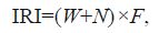
where W is the percent composition by biomass, N is the percent composition by number, and F is the percent frequency of occurrence.
Using equations from the literature, phytoplankton cell volume and biomass were calculated (Strathmann, 1967; Strickland, 1970; Sun et al., 1999) . Zooplankton specimens were weighed and biomass were calculated using equationsfrom related studies (Iguchi and Ikeda, 1998; Ikeda and Shiga, 1999; Satapoomin, 1999; Zuo et al., 2008) .
The ABC curve method can be used to analyzethe community response to environmental changeand human activities at different times and under different stress situations (Yemane et al., 2005) . The difference between the biomass curve and the abundancecurve is given by the W statistic, which represents the area between them. A negativesign for the W statistic indicates that the biomass curve lies below the abundance curve and suggestsa disturbed community, whereas a positive sign indicates that the biomass curve lies above the abundance curve and is indicative of an undisturbed community (Warwick, 1986; Yemane et al., 2005) . In moderatelydisturbed communities, both curves roughly coincide and the W statistic value is close to zero. Herein, values of the W statistic were used to identifycommunity disturbance in BayuquanPort, and the ABC curves were constructed to examine the ecological characteristics of phytoplankton and zooplankton assemblages. For each survey, the W value for each ABC plot derived from the 15 samplingstations is given.
The effect of environmental factors on the phytoplankton and zooplankton communities was analyzed using CANOCO version 4.5 (Microcomputer Power, Ithaca, NY, USA) . The phytoplankton and zooplanktonspecies data were analyzed using detrended correspondence analysis (DCA) to identify the ordination methods (Hill and Gauch, 1980) .If the maximum gradientlength of the four axes is lower than 3, redundancy analysis (RDA) is appropriate (Peng et al., 2012) . Principal componentanalysis (PCA) can explainmost of the variance of the original multivariate data (Jolliffe, 1986) , so that PCA was used to select the variables that made remarkable and independentcontributions to the phytoplankton and zooplankton communities (Tian et al., 2014) .Only those speciesthat represented >5%of the totalin each sample were included in the analysis ( Leira and Sabater, 2005) . All data were log10 (x+1) transformed before multivariate ordination analysis was conducted. Monte Carlo simulationwas used to test the significance (P<0.05) between the environmental variables and the planktondata in the RDA analysis.
3 RESULT 3.1 Environmental characteristicsThe box plot allowed us to visuallyassess the annual and seasonal variability of SPS, COD, PO4-P, DIN, oil, and Chl-a data (Fig. 2) in Bayuquan Port during the period from 2009 to 2013. The average concentration of SPS over the sampling time was 40.6 mg/L (range, 11.2-94.7 mg/L) . SPS levels were kept at a high level, especially in April 2013, the average concentration of SPS was significantlyhigher compared to these during the survey in April 2009, 2010, and 2012 and October 2011 and 2012 (P<0.01; Fig. 2) . Average concentration of COD was 1.91 mg/L (range, 1.43-3.56mg/L) . The average COD concentration in April 2013 was 3.56 mg/L, which was significantly higher than those of the other five averages in October 2012 (0.027 mg/L) and maximum averages in April 2013 (0.048 mg/L) (Fig. 2) . The average Chl-a concentration over the study period was 3.78 μg/L (range, 0.67-8.12 μg/L. Higher Chl-a concentrations were recorded in April 2013 compared with the other survey periods (Fig. 2) .

|
| Figure 2 Variation of SPS, COD, PO4-P, DIN, Oil and Chl-a in Bayuquan Port during the period 2009-2013 |
During the entire survey, 69 taxa of phytoplankton and 23 taxa of zooplankton were identified. Over 80% and 60% of the taxa were diatoms and copepods, respectively; these groups were the most dominant taxa in the total population at all stations.Meanwhile, our results also reveal that diatoms have numerous abundance advantages over dinoflagellates throughout the five year investigation period.
The dominanttaxa based on IRI values which is above 1 000 show that the diatom genus Coscinodiscus were the most frequent types of phytoplankton in the study area, and they included Coscinodiscus subtilis, C. gigas, C. asteromphalus, C. radiatus, C. granii, C. oculusiridis, and C. subtilis. The sum of the dominant taxaoccurred in very high abundances and accounted for>55% to the total phytoplankton population in each survey period. Massive blooms of Chaetoceros lorenzianus, Melosira sulcata, Skeletonema costatum, Eucampia cornuta, and Pseudo-nitz schia delicatissima occurred during April and October 2012 and April 2013, and these bloom species were the most abundant speciesat each station in the study area during the red tide (Fig. 3) . The harmful algal blooms (HAB) species M. sulcata, S. costatum, and C. lorenzi anus accounted for65% of the total population in April 2012, whereas C. lorenzianus, P. delicatissima, and E. cornuta accounted for 56% of the total populationin October 2012 (Fig. 3) . S. costatum also caused a HAB in April 2013, accounting for 86% to the total abundances (Fig. 3) .

|
| Figure 3 Contributions (%) of five dominant species which caused red tides to the total abundance of phytoplankton community in different periods |
The average total abundance valuesof phytoplankton during April and October 2012 and total abundances April 2013 were 7 157.20×10⁴, 3 919.66×10⁴, and 3311.66×104 cells/m3, respectively; these values were significantly higher than those in April 2009 and 2010 and October 2011 (P<0.01; Fig. 4) . HAB species accounted for more than 56% of total phytoplankton abundance in April and October 2012 and April 2013.

|
| Figure 4 Distribution of the phytoplankton and zooplankton abundance in different periods during 2009-2013 in the study area |
Among the zooplankton taxa, Paracalanus parvus, Acartia clausi, Oithona similes, Paracalanus crassirostris, Acartia hongi, nauplius larvae, copepodite, Oikopleura dioica, and Sagitta crassa were the most abundantduring the entirestudy period. The copepods clearly dominatedthe zooplankton community, with the various life cycle stages (adults, nauplius larvae, and copepodite) in the samples accounting for more than 85% of the totalnumber of zooplankton in each survey. After copepods, the other dominant groups were O. dioica and S. crassa, in which S. crassa was dominant in terms of biomass.
Zooplankton abundanceranged from 179.36 (April 2013) to 11 978.75 ind/m3 (April 2012) during the survey period (Fig. 4) . Average total abundance of zooplanktonin April 2012 was significantly higher than that of the other five samplingperiods (P<0.01; Figs. 1-4) . The abundance of zooplankton in April 2013 was significantly lower than that of the other five samplingperiods (P<0.01) .
3.3 Characteristics of the ABC curveFor the phytoplankton community in April 2009, the abundance curve was above the biomasscurve in some places, and the W statistic was negative.In April 2013, the W statistic also was negative (Fig. 5) .In the other four surveys (April 2010; October 2011; April 2012; October2012) , the biomasscurves were above the abundancecurves and the value of W was positive. For zooplankton, with the exception of October 2010 andApril 2012, the value of W was positive (Fig. 6) .The curves roughly coincided for zooplankton community in the October 2010 and April 2013 surveys. In April 2012, the abundance curve overhung the biomass curve. For the other three surveys, the biomass curves were above the abundance curves and had small positive W values.

|
| Figure 5 The ABC curves and W statistic of phytoplankton community in April of 2009 and 2013 |

|
| Figure 6 The ABC curves and W statistic of zooplankton community in October, 2011 and April, 2012 |
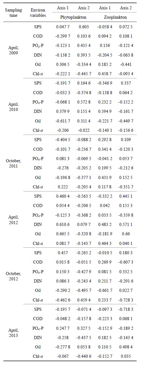
The PCA results for the phytoplankton community are given in Table 1. In April 2009, the first two axes together accounted for 60.2% of the total variance of the data set. Based on these results, we used the first two axes as the principal component axes. Axis 1 was correlated positively with oil and negatively with COD, and axis 2 positively with SPS, PO4-P, and DIN and negatively with Chl-a (Table 1). In April 2010, we used the first two axes as the principal component axes, as they accountedfor 64.1% of the total variation. Axis 1 was correlated positivelywith DIN and negatively with Chl-a and oil (oilhad the strongest correlation) ; axis 2 showed positive correlation with SPS, PO4-P, DIN, and oil (PO4-P had the strongest correlation) and negative with COD and Chl-a (Table 1) . In October 2011, the first two axes together accounted for 46.0% of the total variance of the data set. Axis 1 was y correlated positivelwith Chl-a and negatively with SPS and DIN; axis 2 showed negative correlations with all environmental variables, with the strongest correlation for oil (Table 1) . In April 2012, the first two axes together accountedfor 60.5% of the total varianceof the data set. Axis 1 was correlated positively with SPS, DIN, and oil, and axis 2 negatively with all environmental variables (SPS had the strongest correlation) except for DIN (positive; Table 1) . In October2012, the first two axes together accountedfor 88.4% of the totalvariance of the data set. Axis 1 had a large positivecoeffcient for SPS and a large negativecoeffcient for Chl-a; axis 2was correlated negatively with all environmental variables (oil had the strongest correlation) except for Chl-a (positive; Table 1) . In April 2013, the first two axes togetheraccounted for 77.7%of the total variance of the data set. Axis 1 was correlated negatively with all environmental variables (oil had the strongestcorrelation) except for PO4-P (positive) ; axis 2 had large negativecoeffcients for DIN and Chl-a and a large positivecoeffcient for PO4-P (Table 1) .
|
The PCA results for the zooplankton community are also given in Table 1. In April 2009, the first two axes explained 68.7% of the variance. Therefore, we considered only the first two axes. Axis 1 had a large positive coefficient for Chl-a, and axis 2 was strongly negatively correlatedwith oil (Table 1) . In April 2010, the first two axes explained70.8% of the variance. Axis 1 had a strong positivecoeffcient for DIN, and axis2 was strongly correlated negatively with oil (Table 1) . In October 2011, more than half of the total system variability (98.2%) was due to the first axis (56.7%) . Axis 1 had strong positive coeffcients for COD and oil, and axis 2 was strongly correlated negatively with Chl-a (Table 1) . In April 2012, the first two axes explained 74.4% of the variance. Axis 1 had large positive coeffcients for DIN and Chl-a (DIN had the strongest correlation) , and axis 2 was strongly and positively correlated with oil, DIN, and SPS (oil had the strongestcorrelation) (Table 1) . In October 2012, the first two axes explained86% of the variance. Axis 1 had a strong negativecoeffcient for oil, and axis 2 was stronglyand negatively correlated with Chl-a and COD (Chl-a had the strongest correlation) (Table 1) . In April2013, more than half of the total syste m variability (96.8%) was due to the first axis (54.8%) Axis 1 had a large negative coeffcient for COD and a large positive coeffcient for DIN, and axis 2 had a strong negativecoeffcient for SPS and a large positive coeffcient for oil (Table 1) .
3.5 Relationships between plankton and environmentalfactorsRDA is a way to visualizecorrelations between the phytoplankton community and environmental variables and years (Fig. 7) .In April 2009, 72.3% of the cumulativevariance of the species-environment relationship was represented by the first two axes. All canonical axes accounted for 49.8% of the variation in the phytoplankton data.DIN concentration was related positively to the abundanceof S. costatum. In April 2010, 75.2% of the cumulative variance of the species-environment relationship was represented by the first two axes. All canonical axes accounted for 56.2% of the variationin the phytoplankton data. Oil concentration was positively relatedto abundance of Chaetoceros debilis and negatively related to the abundance of both Biddulphia biddulphiana and Chaetoceros castracanei. In October 2011, 56.2% of the cumulativevariance of the species-environment relationship was represented by the first two axes. All canonical axes accounted for 44.2% of the variation in the phytoplankton data. Oil and SPS concentrations were positively correlated with Eucampia zodiacus abundance. DIN concentration was positively and negatively correlated with Coscinodiscus sp. and E. zodiacus, respectively. In April 2012, 75.2% of the cumulative varianceof the species-environmentrelationship was represented by the first two axes. All canonical axes accounted for 62.4% of the variation in the phytoplankton data.DIN concentration was positively related to the abundance of Guinardia delicatula. In October2012, 86.2% of the cumulative variance of the species-environment relationship was represented by the first two axes. All canonical axes accounted for 63.8% of the variationin the phytoplankton data. Chl-a concentration was related positively to the abundanceof Chaetoceros curvisetus.In April 2013, 76.4% of the cumulative variance of the species-environment relationship was represented by the first two axes. All canonicalaxes accounted for 49.7% of the variationin the phytoplankton data. Chl-a concentrationwas positively relatedto abundances of both P. delicatissima and Thalassiosira sp.

|
| Figure 7 Ordination biplot of environmental variables and phytoplankton species assemblages obtained by RDA during the survey time |
Figure 8 shows the RDA ordination resultsfor zooplankton functional groups and environmental factors. In April 2009, the eigenvalues for RDA axis 1 (0.210) and RDA axis 2 (0.079) explained 72.8% of the varianceof the species-environment relationship. All canonicalaxes accounted for 39.7% of the variation in the zooplankton data. Chl-a concentrationwas related positively to the abundanceof copepodite. In April 2010, the eigenvalues for RDA axis 1 (0.239) and RDA axis 2 (0.130) explained81.0% of the variance of the species-environment relationship. All canonical axes accountedfor 45.6% of the variation in the zooplankton data. Oil concentration was correlated positively with A cartia clausi abundance. In October2011, the eigenvalues for RDA axis 1 (0.316) and RDA axis 2 (0.074) explained 81.8% of the varianceof the species-environment relationship. All canonicalaxes accounted for 47.6% of the variation in the zooplankton data. Oil and SPS concentration were positively correlated with Acartia bifilosa abundance and negativelyto P. parvus abundance, respectively. In April 2012, the eigenvalues for RDA axis 1 (0.241) and RDA axis 2 (0.176) explained 84.1% of the varianceof the species-environment relationship. All canonical axes accounted for 49.6% of the variationin the zooplankton data. In October 2012, the eigenvalues for RDA axis 1 (0.402) and RDA axis 2 (0.296) explained 85.6% of the variance of the species-environment relationship. All canonical axes accounted for 81.6% of the variation in the zooplankton data. In April 2013, the eigenvalues for RDA axis 1 (0.192) and RDA axis 2 (0.132) explained 40.3% of the variance of the species-environment relationship.

|
| Figure 8 Ordination biplot of environmental variables and zooplankton species assemblages obtained by RDA during 2009-2013 |
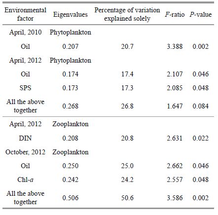
Based on the RDA results, different environmental variables explainedthe variability in the phytoplankton and zooplankton composition, with partialRDA in April 2010 and 2012 and October2012, respectively (Fig. 9; Table 2) . In April 2010, oil had a significant (P<0.05, Monte Carlo permutation test) relationship with the phytoplankton community, whereasin April 2012 the significant environmental variables were oil and SPS. In April 2010 and 2012, Monte Carlo permutation testingrevealed a significant correlation between the DIN concentration and the zooplankton community (P<0.05) . In October 2012, RDA with forward selectionshowed that oil (F=2.662, P=0.046) and Chl-a (F=2.557, P=0.048) explained the variability in the zooplankton community composition.

|
| Figure 9 Correlation plots ofthe partial RDA on the relationship between the environmental variables and plankton taxa |
|
Variation partitioning analysis of the partial RDA was performedto estimate the influenceof each significant variable (Zhang et al., 2011) . The results showed that in April 2010 oil explained 20.7% of the phytoplankton communityvariation (Fig. 9; Table 2) . In April 2012, oil and SPS individually explained 17.4% and 17.3% of the phytoplankton variation, respectively (Fig. 9; Table 2) . DIN concentration explained 17.2% and 20.8% of the zooplankton community variationwithout the other environmental variables in April 2010 and 2012, respectively (Table 2) . In October 2012, oil alone explained 25.0% of the phytoplankton variation, whereas Chl-a explained 24.2% of the zoop lankton variation (Fig. 9; Table 2) .
The variation in plankton composition could be summarized on the first two axes of the partialRDA (Fig. 9) . In April 2010, the dominant speciesof phytoplankton (C. curvisetus, Chaetoceros subsecundus, and C. lorenzianus) were locatedon the right-hand side of the biplot, and they were negatively correlated significantly with oil. In April 2012, the dominant species of phytoplankton were M. sulcata, S. costatum, and C. lorenzianus, which were correlated positively with SPS and oil; Schroderella delicatula was correlated stronglywith axis 2 and negatively correlated with oil. In April 2010, the dominant species of zooplankton were P. parvus, copepodite, and A. clausi. P. parvus was correlated positively with DIN and copepodite, and A. clausi was significantlycorrelated with axis 2. In April 2012, the P. parvus. Oil was correlated positively with O. dioica and negatively with nauplius larvaeand P. parvus.Chl-a was correlated positively with P. parvus and negatively with O. dioica and nauplius larvae.
4 DISCUSSION 4.1 Environmental characteristics of Bayuquan PortLiaodong Bay, especially the Bayuquan Port area, has been affected strongly by various anthropogenic pressures. In the last three decades, the water quality of Yingkou Bay has deteriorated dramatically because of urbanization and industrialand port development. The Bohai Sea received0.8 billion tons of industrial sewage water in 1998 (State Ocean Administration, 2000) , and today Bohai Bay receivesabout 1 billiontons of wastewater each year (Duan et al., 2010) . The main rivers that empty directlyinto Liaodong Bay include the Liaohe, Daliaohe, Dalinghe, Xiaolinghe, and Shuangtaizihe, which carry anthropogenic materials as well as nutrients andsuspended solids, thereby increasing human impacts on water quality in the bay. This riverine input is considered the main source of nutrients (Zhang et al., 2004; Wang et al., 2009; Duan et al., 2010) in the bay, and Wang et al. (2009) reported that Liaohe River was mainly responsible for the eutrophication of LiaodongBay. In our study, the average DIN concentration was 0.763 mg/L, which exceeds the guideline (TN>0.5 mg/L) for eutrophic status (Twist et al., 1998) ; the concentration was only lower than the guideline value in April 2013 (0.131 mg/L) , possibly due to decreased river runoff or regulated discharge of industrial sewage water. The mean PO4-P concentrations during April 2009 and October 2011 and 2012 were 0.031, 0.017, and 0.027 mg/L, respectively, which are close to or beyond the benchmark concentration (TP>0.02 mg/L) for eutrophic status (Twist et al., 1998) . These data suggest that this area was a potentia l eutrophication risk for Bayuquan Port. Meanwhile, red tides, which are linked closely to eutrophication, have been occurring more frequently and spreadingubiquitously in recent years (Sündermann and Feng, 2004) .In addition, SPS levels were high during the survey period in the Bayuquan Port area. Reasons for thehigh concentration of SPS include sedimentresuspension due to wind-induced waves, port dredging, and ocean engineering projects (e.g., reclamation projects and breakwater construction) . High SPS concentrations can have direct or indirect impacts on the planktoncommunity by reducing water transparency, nutrientrelease rate, or adsorption effciency and affectingphytoplankton photosynthesis, which in turn directlyaffects primary consumers (Arruda et al., 1983; Bilotta and Brazier, 2008) . Additionally, hydrological conditions changing, such as sea surfacetemperature and wind speed, would significantly affect the abundanceand distribution of diatoms and dinoflagellates and also possibly increase the occurrence of HAB species (Reid et al., 1998; Moore et al., 2009; Hallegraeff, 2010; Hinder et al., 2012) . Continuous port construction, long-term sea ice trends along the BayuquanPort, sea temperature and summer windiness conditions have created favorable conditions for the growth of diatomsand harmful algal bloom (Cao et al., 2005; Hinder et al., 2012) . Moreover, the unstable ecosystems lead to a decreasein copepod abundance and biomasscompared to the other parts of the LiaodongBay (Song et al., 2010; Lynam et al., 2011) , and its shows a synergistic positive effect the climate conditions and anthropogenic stresses may benefit outbreaksof jellyfish (Lynam et al., 2011; Condon et al., 2013) .
4.2 Annual and seasonalvariation in phytoplankton and zooplankton communitiesAccording to the particle size, phytoplankton can be dividedinto picophytoplankton (0.2-3μm) , nano-phytoplankton (3-20 μm) and microphytoplankton (20-200 μm) (Hong et al., 1999) .“The specifications for marine biological survey of China” (GB/T 12763.6-2007) providestwo methods to collect phytoplankton (i.e., water samplingand trawl with vertical III plankton net (mesh size: 76 μm) ) , however, mainly relied on microscopic identification methods and the scope of the identification was confined to microphytoplankton, but for picophytoplankton and nanophytoplankton species identification methodhas not yet been specified. Due to fewer phytoplankton species in the northernsea area of China, planktonnet trawl can be have higher effciencycompared with water samplingfor phytoplankton collection, while it is diffcult to trawl to collect picophytoplankton, nanophytoplankton and microphytoplankton with an aperture to achieve.For picophytoplankton and nanophytoplankton investigation only through water sampling and molecular biological identification, but cannot be to determine their number and particle size. This researchis mainly aimed at microphytoplankton which were collected by vertical III plankton net, including some chain nanophytoplankton, and zooplankton investigation also only use plankton net (VerticalI and II) , in orderto link the consistency of phytoplankton and zooplankton investigation and to make full use of the history sample data, and therefore the phytoplankton investigation in this paper can only refer to the planktonnets provided by “The specificationsfor marine biological survey of China” (GB/T 12763.6-2007) .
In April 2009 and 2010 and October2011, phytoplankton abundancearound Bayuquan Port was similar to values reportedfrom previous surveys, such as 132.3×10⁴ and 25.1×10⁴ cell/m3 along the shore of the Bohai Sea in May and October 1998, respectively (Wang, 2003) ; 25.1×10⁴ cell/m3 in the area southeastof Liaodong Bay along Yingkou Port from July to September 2005 (Song et al., 2007) ; and 35.66×10⁴ cell/m3 in the area northof Liaodong Bay in May 2009 (Luan et al., 2009) .However, when red tides occurred in the Bohai Sea from 2009 to 2012, the phytoplankton abundanceincreased sharply (Yin et al., 2014) . From 1998 to May 2003, 49 red tides were observedin the north sea of China; 20 of them occurred in Liaodong Bay, accounting for 41% of the total, and most of them occurrednear the shore of Bayuquan Port (Cao et al., 2005) . From May to October 2012, two red tide eventswere observed in BahaiBay, located in the western part of Bohai Sea, and they were caused by S. costatum, P. delicatissima, Chaetoceros sp., and E. zoodiacus (Yin et al., 2014) . We found similar resultsin our study. All of these data indicate that red tides have increasedin frequency and scalein recent years.Several studies have suggested that the occurrence of red tides is stronglyassociated with human activities in coastal zones, especially the anthropogenic loadingsthat lead to eutrophication (Tang et al., 1998; Sellner et al., 2003) . Eutrophication appears to be the key factorfor development of red tides in coastal and bay waters (Paerl, 1997; Lim et al., 2005; Wang et al., 2008) . In Liaodong Bay, th e mass introduction of nutrients from river runoff, sewage and industrial wastewater, semi-closed water, upwelling relaxation (sediment resuspension) , and otheranthropogenic loadings can invoke eutrophication and lead to red tides.
Bi et al. (2001) reportedthat the average zooplankton abundance in the Bohai Sea was 3841 ind/m3 in the 1950-1960s, which is consistent with our results for April 2009 and 2010 and October 2011 and 2012. Song et al. (2010) reported zooplankton abundance of 17 978 ind/m3 in Yingkou Port from July to September 2005, which is similar to our results for April 2012. Grazing by copepodsis thought to have a significant impact on diatom blooms, sometimes suppressing their deterioration (Tiselius, 1988; Bathmann et al., 1990; Liu et al., 2009) , which in turn can lead to increasedzooplankton abundance such as that seen in April and October 2012 in this study. However, zooplankton abundance in April 2013 was significantly lower than that of the other samplingperiods. This may have been due to the increasedabundance of red tide species and dramatic rise in SPS concentration, which can alter the food web dynamicsand reduce phytoplankton diversity. The resultingchanges in the food chain and feeding environment can lead to fluctuations in the food available for zooplankton.
Nutrient levels play an important role in marine biodiversity and influence competition and community structure in the marineenvironment (Raghukumar and Anil, 2003; Worm et al., 2006; Gaonkar et al., 2010) . In addition, severalstudies speculated that human activities and environmental factorsinfluence the spatialand temporal distributions of the abundance and biomassof aquatic organisms (DelValls et al., 1998; Magni et al., 2005, 2006) .In the present study, the ABC curves and their corresponding W values for the phytoplankton and zooplankton communities indicate the presence of a moderateto high range of pollution in the study area. The plankton communities were affected significantly by external disturbances, suggesting that the environmental variables give increasingly adversepressure to the plankton community aroundcoastal in the Bayuquan Port. The increased levelsof eutrophication and anthropogenic stresses in Liaodong Bay have already affected the abundance of phytoplankton and zooplankton and keeping them in a sharp fluctuation level in the Bayuquan Port.
4.3 Environmentalfactors regulatingthe plankton assemblagesPhytoplankton communitystructure and abundance could make a rapidlyresponse to vary in the environmental factor, and some of them may play a pivotal role in phytoplankton diversification (Peng et al., 2013) .Our results suggestthat the phytoplankton composition, abundance, and succession in Bayuquan Port were strongly influenced by oil, DIN, SPS, PO4-P, and Chl-a, which contributed greatly to axis 1 and axis 2 throughout the study period.The annual and seasonaldynamics of phytoplankton composition and abundance and dominant species were most likely controlled by the environmental conditions of the habitat (Peng et al., 2013) .
According to the RDA, C. debilis, E. zodiacus, B. biddulphiana, and C. castracanei were correlated strongly with oil concentration. The partial RDA results suggestthat the phytoplankton community was affected significantly by the oil and SPS levels in April 2010 and 2012. Furthermore, the abundances of Coscinodiscus sp., G. delicatula, and Stephanopyxis turris were closely associated with high DIN concentration and E. zodiacus was the dominant species in October 2011 and closely associated to the low DIN. C. curvisetus, P. delicatissima, and Thalassiosira sp. abundances also were significantly correlated with high Chl-a concentration. The above results suggest that phytoplankton species use differentstrategies to adapt to the environmental conditions and changes.
It is recognized generally that estuarine/coastal marine red tides are closely linked with the nutrient concentrations in the water column (Anderson et al., 2002; Glibert and Burkholder, 2006) . In our study, the red tide forming diatoms were C. lorenzianus, M. sulcata, S. costatum, E. cornuta, and P. delicatissima, and bloomswere caused by high DIN loadingfrom river runoff and sediment resuspension at Bayuquan Port during April and October 2012 and April 2013. S. costatum is known to be associatedwith high nutrientsconcentrations (Patil and Anil, 2011; Peng et al., 2013) . Furthermore, the environmental factors (oil, SPS, and Chl-a) also contributed to the phytoplankton blooms.
In the presentstudy, the PCA resultssuggest that the zooplankton community in BayuquanPort was strongly influenced by oil, DIN, SPS, and Chl-a during the survey period. The results indicatethat changes in oil, SPS, and Chl-a levels could have a great impact on the zooplankton species (e.g., A. clausi, A. bifilosa, P. parvus, and copepodite) present in Bayuquan Port. The partialRDA results suggest that annual changesin DIN concentration were more pronounced and may have had a greater impact on the zooplankton community in April 2010 and 2012 than during the other samplingperiods. The oil and Chl-a were significantlyassociated with zooplankton composition and abundance. Previous studies have shown that zooplankton play an important role in the phytoplankton community via grazing pressure, thereby affecting its abundanceand biomass (Morales et al., 1991; Dam and Peterson, 1993; Zhang et al., 1995) . Thus, it is most likely that zooplankton abundance increasedin conjunction with algae blooms duringthe surveys in the BayuquanPort. However, the RDA results indicate that an increased SPS concentration can have a negative effect on zooplankton abundance, which may explain the dramatic reduction in zooplankton abundancein April 2013. Based on these findings, we infer that the zooplankton communityin Bayuquan Port was affected strongly by both environmental factors and the phytoplankton community.
5 CONCLUSIONRed tides occur frequently in Bayuquan Port from 2012 to 2013. Eutrophication and high concentrations of suspended solids showed negativeeffects on phytoplanktonand zooplankton community. Zooplankton abundancewas closely associatedwith the phytoplankton communitywhen the red tide occurred. Significant relation was found between plankton communities and some environmental factors e.g., oil, dissolved inorganic nitrogen (DIN) , suspended solids (SPS) , and chlorophyll a (Chl-a) .Generally, eutrophication processes were driven by river runoff and increasedthe SPS levels, which were caused by intensive marineengineering and rapid industrialization and urbanization over the past three decades. These factors have heavily stressedthe marine environment and greatly degradedplankton ecosystemsin Bayuquan Port in LiaodongBay.
Now, port construction has become a key issue for changing coastalport cities in economic and social, but environmental terms serves as a new challenge for them. How can the potential and foreseeable coastal contamination problemsin the process of port reconstruction in waterfront be resolved? On the basis of the scientific assessment and protection of the marine environment along the BayuquanPort of Liaodong Bay, Bohai Sea, the following goals need to be addressed:
First, we should be learning the experienced of port construction in the developedcountries. Second, to further strengthenenvironmental supervision in the port waters, promote environmental remediation and ecological restoration. Third, in additionto the efforts of planners, designers and local government, the process needs multidisciplinary efforts from project feasibility studiesin academia at home and abroad to focus on the marine environmental impacts of the port redevelopment, in line with sustainable development, to seek multiple appropriate redevelopment models. Furthermore, we would pay more attention to the particles size structure of the planktoncommunity under different marine environmental conditions in the harbor water area in the future, as well as distribution and succession of alien invasive micro-organisms, and the interaction between environmental factors and outbreaks of jellyfish deserving of further study in experimental and in situ conditions.
| Ananthan G A, Sampathkumar P, Soundarapandian P, Kannan L, 2005. Observation on environmental characteristics of Ariyankuppam estuary and Veerampattinam coast of Pondicherry, India. J. Aqua. Biol., 19 (2) : 67 –72. |
| Anderson D M, Glibert P M, Burkholder J M, 2002. Harmful algal blooms and eutrophication: nutrient sources, composition, and consequences. Estuaries, 25 (4) : 704 –726. |
| Arruda J A, Marzolf G R, Faulk R T, 1983. The role of suspended sediments in the nutrition of zooplankton in turbid reservoirs. Ecology, 64 (5) : 1225 –1235. Doi: 10.2307/1937831 |
| Bathmann U V, Noji T T, von Bodungen B, 1990. Copepod grazing potential in late winter in the Norwegian Sea-a factor in the control of spring phytoplankton growth? Mar. Ecol. Prog. Ser., 60 : 225 –233. Doi: 10.3354/meps060225 |
| Bi H S, Sun S, Gao S W, Zhang G T, 2001. The ecological characteristics of zooplankton community in the Bohai Sea II: the distribution of copepoda abundance and seasonal dynamics. Acta Ecologica Sinica, 21 (2) : 177 –185. |
| Bilotta G S, Brazier R E, 2008. Understanding the influence of suspended solids on water quality and aquatic biota. Water. Res., 42 (12) : 2849 –2861. |
| Buruaem L M, Hortellani M A, Sarkis J E, Costa-Lotufo L V, Abessa D M S, 2012. Contamination of port zone sediments by metals from Large Marine Ecosystems of Brazil. Mar. Pollut. Bull., 64 (3) : 479 –488. Doi: 10.1016/j.marpolbul.2012.01.017 |
| Cao C H, Huang J, Guo M K, Jiang C B, Li P S, 2005. The analysis of red tide and environmental factor in Bayuquan, Liaodong Bay. Mar ine Forecasts, 22 (2) : 1 –6. |
| Casé M, Leça E E, Leitão S N, Sant'Anna E E, Schwamborn R, de Moraes Junior A T, 2008. Plankton community as an indicator of water quality in tropical shrimp culture ponds. Mar. Pollut. Bull., 56 (7) : 1343 –1352. Doi: 10.1016/j.marpolbul.2008.02.008 |
| Condon R H, Duarte C M, Pitt K A, et al, 2013. Recurrent jellyfish blooms are a consequence of global oscillations. Proc. Natl. Acad. Sci. U. S. A., 110 (3) : 1000 –1005. Doi: 10.1073/pnas.1210920110 |
| Dam H G, Peterson W T, 1993. Seasonal contrasts in the diel vertical distribution, feeding behavior, and grazing impact of the copepod Temora longicornis in Long Island Sound. J. Mar. Res., 51 (3) : 561 –594. Doi: 10.1357/0022240933223972 |
| Darbra R M, Ronza A, Casal J, Stojanovic T A, Wooldridge C, 2004. The self diagnosis method: a new methodology to assess environmental management in sea ports. Mar. Pollut. Bull., 48 (5-6) : 420 –428. Doi: 10.1016/j.marpolbul.2003.10.023 |
| Debelius B, Forja J M, DelValls Á, Lubián L M, 2009. Toxicity and bioaccumulation of copper and lead in five marine microalgae. Ecotox. Environ. Safe., 72 (5) : 1503 –1513. Doi: 10.1016/j.ecoenv.2009.04.006 |
| DelValls T A, Conradi M, Garcia-Adiego E, Forja J M, Gómez-Parra A, 1998. Analysis of macrobenthic community structure in relation to different environmental sources of contamination in two littoral ecosystems from the Gulf of Cádiz (SW Spain). Hydrobiologia, 385 (1-3) : 59 –70. |
| Duan L Q, Song J M, Li X G, Yuan H M, Xu S S, 2010. Distribution of selenium and its relationship to the ecoenvironment in Bohai Bay seawater. Mar. Chem., 121 (1-4) : 87 –99. |
| Ferraro S P, Swartz R C, Cole F A, Schults D W, 1991. Temporal changes in the benthos along a pollution gradient: discriminating the effect of natural phenomena from sewage-industrial wastewater effects. Estuar. Coast. Shelf S ci., 33 (4) : 383 –407. |
| Fietz S, Kobanova G, Izmest'eva L, Nicklisch A, 2005. Regional, vertical and seasonal distribution of phytoplankton and photosynthetic pigments in Lake Baikal. J. Plankton Res., 27 (8) : 793 –810. Doi: 10.1093/plankt/fbi054 |
| Gao S L, Liu N, Sun L H, 1994. The construction and its development of the overseas transport system in northeast China. Chin. Geogr. Sci., 4 (1) : 19 –30. Doi: 10.1007/BF02664947 |
| Gaonkar C A, Krishnamurthy V, Anil A C, 2010. Changes in the abundance and composition of zooplankton from the ports of Mumbai, India. Environ. Monit. Assess., 168 (1-4) : 179 –194. |
| GB 17378.6-2007. The specification for marine monitoring—Part 6: organism analysis. China Standards Press, Beijing. p.1-79. (in Chinese) |
| GB 17378.4-2007. The specification for marine monitoring—Part 4: seawater analysis. China Standards Press, Beijing. p.1-162. (in Chinese) |
| GB 12763.6-2007. The specifications for marine biological survey of China—Part 6: marine biological survey. China Standard Press, Beijing. p.1-157. (in Chinese) |
| Glibert P M, Burkholder J M, 2006. The complex relationships between increases in fertilization of the earth, coastal eutrophication and proliferation of harmful algal blooms. Ecology of Harmful Algae. Springer, Berlin Heidelberg (341) : 354 . |
| HallegraeffG M, 2010. Ocean climate change, phytoplankton community responses, and harmful algal blooms: A formidable predictive challenge. J. Phycol., 46 (2) : 220 –235. Doi: 10.1111/jpy.2010.46.issue-2 |
| Hassan F M, Kathim N F, Hussein F H, 2008. Effect of chemical and physical properties of river water in Shatt Al-Hilla on phytoplankton communities. J. Chem., 5 (2) : 323 –330. |
| Herrera-Silveira J A, Morales-Ojeda S M, 2009. Evaluation of the health status of a coastal ecosystem in southeast Mexico: assessment of water quality, phytoplankton and submerged aquatic vegetation. Mar. Pollut. Bull., 59 (1-3) : 72 –86. Doi: 10.1016/j.marpolbul.2008.11.017 |
| Hill M O, Gauch Jr H E J, 1980. Detrended correspondence analysis: an improved ordination technique. Vegetatio, 42 (1-3) : 47 –58. Doi: 10.1007/BF00048870 |
| Hinder S L, Hays G C, Edwards M, Roberts E C, Walne A W, Gravenor M B, 2012. Changes in marine dinoflagellate and diatom abundance under climate change. Nat. Climate Change, 2 (4) : 271 –275. Doi: 10.1038/nclimate1388 |
| Hong H S, Shang S L, Huang B Q, 1999. An estimate on external fluxes of phosphorus and its environmental significance in Xiamen Western Sea. Mar. Pollut. Bull., 39 (1-2) : 200 –204. |
| Iguchi N, Ikeda T, 1998. Elemental composition (C, H, N) of the euphausiid Euphausia pacifica in Toyama Bay, southern Japan Sea. Plankton Biol. Ecol., 45 (1) : 79 –84. |
| Ikeda T, Shiga N, 1999. Production, metabolism and production/biomass (P / B) ratio of Themisto japonica (Crustacea: Amphipoda) in Toyama Bay, southern Japan Sea. J. Plankton Res., 21 (2) : 299 –308. Doi: 10.1093/plankt/21.2.299 |
| Jiang Z B, Zhu X Y, Gao Y, Chen Q Z, Zeng J N, Zhu G H, 2013. Spatio-temporal distribution of net-collected phytoplankton community and its response to marine exploitation in Xiangshan Bay. Chin. J. Oceanol. Limnol., 31 (4) : 762 –773. Doi: 10.1007/s00343-013-2206-z |
| Jolliffe I T. 1986. Principal Component Analysis. Springer, New York, Berlin, Germany. p.1-7. |
| Karthik R, Arun Kumar M, Sai Elangovan S, Siva Sankar R, Padmavati G. 2012. Phytoplankton abundance and diversity in the coastal waters of Port Blair, South Andaman Island in relation to environmental variables. J. Mar. Biol. Oceanogr., 1: 2. |
| Kim M, Hong S H, Won J, Yim U H, Jung J H, Ha S Y, An J G, Joo C, Kim E, Han G M, Baek S, Choi H W, Shim W J, 2013. Petroleum hydrocarbon contaminations in the intertidal seawater after the Hebei Spirit oil spill—effect of tidal cycle on the TPH concentrations and the chromatographic characterization of seawater extracts. Water Res., 47 (2) : 758 –768. Doi: 10.1016/j.watres.2012.10.050 |
| Leira M, Sabater S, 2005. Diatom assemblages distribution in Catalan Rivers, NE Spain, in relation to chemical and physiographical factors. Water Res., 39 (1) : 73 –82. Doi: 10.1016/j.watres.2004.08.034 |
| Lim P T, Usup G, Leaw C P, Ogata T, 2005. First report of Alexandrium taylori and Alexandrium peruvianum (Dinophyceae) in Malaysia waters. Harmful Algae, 4 (2) : 391 –400. Doi: 10.1016/j.hal.2004.07.001 |
| Liu D Y, Keesing J K, Xing Q G, Shi P, 2009. World's largest macroalgal bloom caused by expansion of seaweed aquaculture in China. Mar. Pollut. Bull., 58 (6) : 888 –895. Doi: 10.1016/j.marpolbul.2009.01.013 |
| Luan S, Gong X Z, Shuang X Z, Gao W, Yin B S, Xing Y Z, 2009. Investigation of net-phytoplankton community structure in Liaodong Bay in spring of 2009. Mar. Sci., 36 (5) : 57 –64. |
| Lynam C P, Lilley M K S, Bastian T, Doyle T K, Beggs S E, Hays G C, 2011. Have jellyfish in the Irish Sea benefited from climate change and overfishing?. Global Change Biol, 17 (2) : 767 –782. Doi: 10.1111/gcb.2010.17.issue-2 |
| Magni P, Como S, Montani S, Tsutsumi H, 2006. Interlinked temporal changes in environmental conditions, chemical characteristics of sediments and macrofaunal assemblages in an estuarine intertidal sandflat (Seto Inland Sea, Japan). Mar. Biol., 149 (5) : 1185 –1197. Doi: 10.1007/s00227-006-0298-0 |
| Magni P, Micheletti S, Casu D, Floris A, Giordani G, Petrov A N, De Falco G, Castelli A, 2005. Relationships between chemical characteristics of sediments and macrofaunal communities in the Cabras lagoon (Western Mediterranean, Italy). Hydrobiologia, 550 (1) : 105 –119. Doi: 10.1007/s10750-005-4367-z |
| McGlathery K J, Sundbäck K, Anderson I C, 2007. Eutrophication in shallow coastal bays and lagoons: the role of plants in the coastal filter. Mar. Ecol. Prog. Ser., 348 : 1 –18. Doi: 10.3354/meps07132 |
| Moore S K, Mantua N J, Hickey B M, Trainer V L, 2009. Recent trends in paralytic shellfish toxins in Puget Sound, relationships to climate, and capacity for prediction of toxic events. Harmful Algae, 8 (3) : 463 –477. Doi: 10.1016/j.hal.2008.10.003 |
| Morales C E, Bedo A, Harris R P, Tranter P R G, 1991. Grazing of copepod assemblages in the north-east Atlantic: the importance of the small size fraction. J. Plankton Res., 13 (2) : 455 –472. Doi: 10.1093/plankt/13.2.455 |
| Nowrouzi S, Valavi H, 2011. Effects of environmental factors on phytoplankton abundance and diversity in Kaftar Lake. J. Fish. Aquat. Sci., 6 (2) : 130 –140. Doi: 10.3923/jfas.2011.130.140 |
| Paerl H W, 1997. Coastal eutrophication and harmful algal blooms: importance of atmospheric deposition and groundwater as “new” nitrogen and other nutrient sources. Limnol. Oceanogr., 42 (5) : 1154 –1165. |
| Patil J S, Anil A C, 2011. Variations in phytoplankton community in a monsoon-influenced tropical estuary. Environ. Monit. Assess., 182 (1-4) : 291 –300. Doi: 10.1007/s10661-011-1876-2 |
| Peng C R, Zhang L, Zheng Y Z, Li D H, 2013. Seasonal succession of phytoplankton in response to the variation of environmental factors in the Gaolan River, Three Gorges Reservoir, China. Chin. J. Oceanol. Limnol., 31 (4) : 737 –749. Doi: 10.1007/s00343-013-2165-4 |
| Peng S T, Qin X B, Shi H H, Zhou R, Dai M X, Ding D W, 2012. Distribution and controlling factors of phytoplankton assemblages in a semi-enclosed bay during spring and summer. Mar. Pollut. Bull., 64 (5) : 941 –948. Doi: 10.1016/j.marpolbul.2012.03.004 |
| Pereira C D S, de Souza Abessa D M, Bainy A C D, Zaroni L P, Gasparro M R, Bicego M C, Taniguchi S, Furley T H, de Sousa E C P M, 2007. Integrated assessment of multilevel biomarker responses and chemical analysis in mussels from São Sebastião, São Paulo, Brazil. Environ. Toxicol. Chem., 26 (3) : 462 –469. Doi: 10.1897/06-266R.1 |
| Pinkas L, Oliphant M S, Iverson I L K, 1971. Food habits of albacore, Bluefin tuna, and bonito in California waters. Fish Bull., 152 : 1 –105. |
| Praveena S M, Aris A Z, 2013. A baseline study of tropical coastal water quality in Port Dickson, Strait of Malacca, Malaysia. Mar. Pollut. Bull., 67 (1-2) : 196 –199. Doi: 10.1016/j.marpolbul.2012.11.037 |
| Raghukumar S, Anil A C, 2003. Marine biodiversity and ecosystem functioning: a perspective. Curr. Sci. India, 84 (7) : 884 –892. |
| Reid P C, Edwards M, Hunt H G, Warner A J, 1998. Phytoplankton change in the North Atlantic. Nature, 391 (6667) : 546 . Doi: 10.1038/35290 |
| Riba I, García-Luque E, Blasco J, DelValls T A, 2003. Bioavailability of heavy metals bound to estuarine sediments as a function of pH and salinity values. Chem. Spec. Bioavailab., 15 (4) : 101 –114. Doi: 10.3184/095422903782775163 |
| Rossi N, Jamet J L, 2008. In situ heavy metals (copper, lead and cadmium) in different plankton compartments and suspended particulate matter in two coupled Mediterranean coastal ecosystems (Toulon Bay, France). Mar. Pollut. Bull., 56 (11) : 1862 –1870. Doi: 10.1016/j.marpolbul.2008.07.018 |
| Ruggieri N, Castellano M, Capello M, Maggi S, Povero P, 2011. Seasonal and spatial variability of water quality parameters in the Port of Genoa, Italy, from 2000 to 2007. Mar. Pollut. Bull., 62 (2) : 340 –349. Doi: 10.1016/j.marpolbul.2010.10.006 |
| Sahu B K, Begum M, Khadanga M K, Jha D K, Vinithkumar N V, Kirubagaran R, 2013. Evaluation of significant sources influencing the variation of physico-chemical parameters in Port Blair Bay, South Andaman, India by using multivariate statistics. Mar. Pollut. Bull., 66 (1-2) : 246 –251. Doi: 10.1016/j.marpolbul.2012.09.021 |
| Salmaso N, Braioni M G, 2008. Factors controlling the seasonal development and distribution of the phytoplankton community in the lowland course of a large river in northern Italy (River Adige). Aquat. Ecol., 42 (4) : 533 –545. Doi: 10.1007/s10452-007-9135-x |
| Satapoomin S, 1999. Carbon content of some common tropical Andaman Sea copepods. J. Plankton Res., 21 (11) : 2117 –2123. Doi: 10.1093/plankt/21.11.2117 |
| Sellner K G, Doucette G J, Kirkpatrick G J, 2003. Harmful algal blooms: causes, impacts and detection. J. Ind. Microbiol. Biot., 30 (7) : 383 –406. Doi: 10.1007/s10295-003-0074-9 |
| Shapiro J, 1997. The role of carbon dioxide in the initiation and maintenance of blue-green dominance in lakes. Freshwater Biol., 37 (2) : 307 –323. Doi: 10.1046/j.1365-2427.1997.00164.x |
| Simeonov V, Stratis J A, Samara C, Zachariadis G, Voutsa D, Anthemidis A, Sofoniou M, Kouimtzis Th, 2003. Assessment of the surface water quality in northern Greece. Water Res., 37 (17) : 4119 –4124. Doi: 10.1016/S0043-1354(03)00398-1 |
| Singh K P, Malik A, Mohan D, Sinha S, 2004. Multivariate statistical techniques for the evaluation of spatial and temporal variations in water quality of Gomti River (India) — a case study. Water Res., 38 (18) : 3980 –3992. Doi: 10.1016/j.watres.2004.06.011 |
| Song L, Zhou Z C, Wang N B, Ma Z Q, Xue K, Deng H, Tian J, Yang S, 2007. Phytoplankton diversity of Liaodong Bay and relationship with ocean environmental factors. Mar. Environ. Sci., 26 (4) : 365 –368. |
| Song L, Zhou Z C, Wang N B, Ma Z Q, Xue K, Tian J, Yang S, Wang Z H, Wu J H, 2010. Zooplankton diversity of Liaodong Bay and relationship with oceanic environmental factors. Mar. Sci., 34 (3) : 35 –39. |
| State Ocean Administration. 2000. Bulletin of China Ocean Environmental State at the End of the 20th Century, Beijing, China. (in Chinese) |
| Strathmann R R, 1967. Estimating the organic carbon content of phytoplankton from cell volume or plasma volume. Limnol. Oceanogr., 12 (3) : 411 –418. Doi: 10.4319/lo.1967.12.3.0411 |
| Strickland J D H, 1970. The ecology of the plankton offLa Jolla, California, in the period April through September, 1967. Bull. Scripps Inst. Oceanogr., 17 : 1 –10. |
| Sun J, Liu D Y, Qian S B, 1999. Study on phytoplankton biomass I: phytoplankton measurement biomass from cell volume or plasma volume. Acta Oceanol. Sin., 21 (2) : 75 –85. |
| Sündermann J, Feng S Z, 2004. Analysis and modelling of the Bohai sea ecosystem — a joint German-Chinese study. J. Marine Syst., 44 (3-4) : 127 –140. Doi: 10.1016/j.jmarsys.2003.09.006 |
| Tang D L, Ni I H, Müller-Karger F E, Liu Z J, 1998. Analysis of annual and spatial patterns of CZCS-derived pigment concentration on the continental shelf of China. Cont. Shelf Res., 18 (12) : 1493 –1515. Doi: 10.1016/S0278-4343(98)00039-9 |
| Tang Q, 2004. Study on Ecosystem Dynamics in Coastal Ocean. III, Atlas of the Resources and Environment in the East China Sea and the Yellow Sea Ecosystem. Beijing: Science Press, Beijing, China. |
| Tas B, Gonulol A, 2007. An ecologic and taxonomic study on phytoplankton of a shallow lake, Turkey. J. Environ. Biol., 28 (2) : 439 –445. |
| Tian Y Q, Huang B Q, Yu C C, Chen N W, Hong H S, 2014. Dynamics of phytoplankton communities in the Jiangdong Reservoir of Jiulong River, Fujian, South China. Chin. J. Oceanol. Limnol., 32 (2) : 255 –265. Doi: 10.1007/s00343-014-3158-7 |
| Tiselius P, 1988. Effects of diurnal feeding rhythms, species composition and vertical migration on the grazing impact of calanoid copepods in the Skagerrak and Kattegat. Ophelia, 28 (3) : 215 –230. Doi: 10.1080/00785326.1988.10430814 |
| Twist H, Edwards A C, Codd G A, 1998. Algal growth responses to waters of contrasting tributaries of the river Dee, north-east Scotland. Water Res., 32 (8) : 2471 –2479. Doi: 10.1016/S0043-1354(97)00450-8 |
| Wang J, 2003. Species composition and quantity variation of phytoplankton in inshore waters of the Bohai Sea. Mar. Fish. Res., 24 (4) : 44 –50. |
| Wang R F, Yu G Z, 1997. The open port system in northeast China. Chin. Geogr. Sci., 7 (3) : 270 –277. Doi: 10.1007/s11769-997-0054-5 |
| Wang S F, Tang D L, He F L, Fukuyo Y, Azanza R V, 2008. Occurrences of harmful algal blooms (HABs) associated with ocean environments in the South China Sea. Hydrobiologia, 596 (1) : 79 –93. Doi: 10.1007/s10750-007-9059-4 |
| Wang X L, Cui Z G, Guo Q, Han X R, Wang J T, 2009. Distribution of nutrients and eutrophication assessment in the Bohai Sea of China. Chin. J. Oceanol. Limnol., 27 (1) : 177 –183. Doi: 10.1007/s00343-009-0177-x |
| Wang X, Xu Z F, Zhou X J, 1995. Benthic animal survey in Yantai inshores. Chin. J. Ecol., 14 (1) : 6 –10. |
| Warwick R M, 1986. A new method for detecting pollution effects on marine macrobenthic communities. Mar. Biol., 92 (4) : 557 –562. Doi: 10.1007/BF00392515 |
| Worm B, Barbier E B, Beaumont N, Duffy J E, Folke C, Halpem B S, Jackson J B C, Lotze H K, Micheli F, Palumbi S R, Sala E, Selkoe K A, Stachowicz J J, Watson R, 2006. Impacts of biodiversity loss on ocean ecosystem services. Science, 314 (5800) : 787 –790. Doi: 10.1126/science.1132294 |
| Wu M L, Wang Y S, Sun C C, Wang H L, Dong J D, Yin J, Han S H, 2010. Identification of coastal water quality by statistical analysis methods in Daya Bay, South China Sea. Mar. Pollut. Bull., 60 (6) : 852 –860. Doi: 10.1016/j.marpolbul.2010.01.007 |
| Yemane D, Field J G, Leslie R W, 2005. Exploring the effects of fishing on fish assemblages using Abundance Biomass Comparison (ABC) curves. ICES J. Mar. Sci., 62 (3) : 374 –379. Doi: 10.1016/j.icesjms.2005.01.009 |
| Yin C L, Zhang Q F, Liu Y, Cui J, He R, 2014. Red tide occurrence and eutrophication status in the red tide monitoring area of Bohai Bay in 2012. Transactions of Oceanology Limnology, 37 (1) : 137 –142. |
| Zhang J, Yu Z G, Raabe T, Liu S M, Starke A, Zou L, Gao H W, Brockmann U, 2004. Dynamics of inorganic nutrient species in the Bohai seawaters. J. Marine Syst., 44 (3-4) : 189 –212. Doi: 10.1016/j.jmarsys.2003.09.010 |
| Zhang J C, Zeng G M, Chen Y N, Yu M, Yu Z, Li H, Yu Y, Huang H L, 2011. Effects of physico-chemical parameters on the bacterial and fungal communities during agricultural waste composting. Bioresour. Technol., 102 (3) : 2950 –2956. Doi: 10.1016/j.biortech.2010.11.089 |
| Zhang X, Dam H G, White J R, Roman M R, 1995. Latitudinal variations in mesozooplankton grazing and metabolism in the central tropical Pacific during the U. S. JGOFS EqPac study. Deep Sea Res earch P ar t II: Topical Studies in Oceanography, 42 (2-3) : 695 –714. |
| Zheng G X, Li Y J, Qi L L, Liu X M, Wang H, Yu S P, Wang Y H, 2014. Marine phytoplankton motility sensor integrated into a microfluidic chip for high-throughput pollutant toxicity assessment. Mar. Pollut. Bull., 84 (1-2) : 147 –154. Doi: 10.1016/j.marpolbul.2014.05.019 |
| Zuo T, Wang J, Jin X S, Li Z Y, Tang Q S, 2008. Biomass size spectra of net plankton in the adjacent area near the Yangtze River Estuary in spring. Acta Ecologica Sinica, 28 (3) : 1174 –1182. Doi: 10.1016/S1872-2032(08)60037-2 |