 2016, 34
Institute of Oceanology, Chinese Academy of Sciences
Article Information
- Haijiao LIU(刘海娇), Bing XUE(薛冰), Yuanyuan FENG(冯媛媛), Rui ZHANG(张锐), Mianrun CHEN(陈绵润), Jun SUN(孙军)
- Size-fractionated Chlorophyll a biomass in the northern South China Sea in summer 2014
- Journal of Oceanology and Limnology, 34(4): 672-682
- http://dx.doi.org/10.1007/s00343-016-5017-1
Article History
- Received: Jan. 21, 2015
- Accepted: Apr. 14, 2015


2. Tianjin Key Laboratory of Marine Resources and Chemistry, Tianjin University of Science and Technology, Tianjin 300457, China;
3. State Key Laboratory of Marine Environmental Science and the Institute of Marine Microbes and Ecospheres, Xiamen University, Xiamen 361102, China;
4. Institute of South China Sea Planning and Environment, State Oceanic Administration (SOA), Guangzhou 510300, China
The South China Sea (SCS) is the largest semi-SCS can be traced back to the 1970s. Guo et al. (1978) and Ye et al. (1983) led preliminary studies of netz-closed deep marginal sea, covering an area of 3 500 000 km2. Due to monsoons, it is characterized by extreme seasonalvariations (Su, 2005; Hu et al., 2014) . There are complexbiogeographic and hydrological featuresin the northern South China Sea (NSCS), affected by coastal eutrophic water and deep basin oligotrophic water (Gong et al., 1992) .
Investigations on phytoplankton distribution in the SCS can be traced back to the 1970s. Guo et al. (1978) and Ye et al. (1983) led preliminary studies of netz-phytoplankton, whereas Le et al. (2006) and Sun et al. (2007) reported phytoplankton community and spatial patterns. Peng et al. (2006) elucidated the dynamics of phytoplankton growth by nutrientenrichment. Furthermore, Chen et al. (2006) studied the features of phytoplankton communities in an upwellingregion and warm eddy waters, respectively. More recently, Ma and Sun (2014) depictedthe phytoplankton community and its controlling factors in the summer and winter. Phytoplankton assemblages of small-scale regional areas (Nansha Island, Daya Bay, Zhujiang (Pearl) River) have also been surveyed (Song et al., 2002; Li et al., 2005, 2008; Wang et al., 2006, 2009; Ho et al., 2010; Qiu et al., 2010; Shen et al., 2010) .
The marine chlorophyll a (Chl a) content represents the standing stock of phytoplankton in a region (Le and Ning, 2006) , with the Chl a abundance and pattern denoting the structure and density of the phytoplankton community (Zhou et al., 2004) . Previous studieshave reported the distribution of total Chl a (Ning et al., 2004; Zhao et al., 2005; Zhang et al., 2007; Le et al., 2008; Lin et al., 2010) , and size-fractionated Chl a (Liu et al., 1998; Che et al., 2012) in the SCS. In oligotrophic oceans, small Chl a fractions are major contributors to phytoplankton biomass and the microbialfood web (Berman et al., 1986; Azov, 1991; Polat and Aka, 2007) . Indeed, up to 50% of total Chl a biomass was contributed by picoplanktonin some regions (Gieskes et al., 1979; Platt et al., 1983; Odate and Maita, 1989; Iriarte and Purdie, 1994) . However, large temporal-spatial heterogeneity has been observedin Chl a structure in the aforementioned studies. Diurnal fluctuations in Chl a concentration may have coincided with diurnal photosynthesis periodicity, and this relationship can be numerically estimated (Shimada, 1958; Yentsch and Ryther, 2003) . Chl a consumed by zooplankton can be degraded into phaeopigments and non-fluorescent materials (Helling and Baars, 1985) . Chl a degradationinto phaeopigment is often caused by zooplankton grazing, bacterial activity, autolyticcell lysis and cell sinking. Phaeopigment was abundantly distributed in sediments (Bianchi et al., 1991; Fundel et al., 1998; Zhao et al., 2010) . Widevariety of degradation productscan be acted as indicatorsof grazing activity ( Jeffrey, 1980) . The sinking fecal materials also can be reingested by bathypelagic predators locatedat differed depths and was preserved in their guts (Lorenzen et al., 1983) . Hence, proportions of phaeopigments can be used to interpret carbon transferand transmission effciency in the marine carbon cycle.
In this study, the spatial distribution and variation of size-fractionated Chl a and phaeopigment in the NSCS were examined.Special emphasis was placed on determining the heterogeneity of different sized Chl a and observingthe Chl a dynamics at two mooring stations. Time-series studies at two stations were also conducted, to understand the diurnal variations in Chl a biomass. In addition, the relationship between the distribution of the size-fractionated Chl a concentration and dissolvedinorganic nutrient concentrations was studied. The information presented fills our knowledge gap in understanding the spatial and temporal variations in size fractionated Chl a and phaeopigment concentrations, and their relationship with environmental controllers of biological characteristics in the NSCS.
2 MATERIAL AND METHOD 2.1 Sample collection and analysisField routine sampling was conductedduring the summer cruise of the R/V Shi Yan 1 in August/ September 2014. The elevensampling stations are shown in Fig. 1 includingtwo times-series stations (SEATS and J4) . The bottom depths from the nearshore to offshore stations were 28 m, 46 m, 71 m, 76 m, 106 m, 141m, 737 m, 2 176 m, 2 671 m, 3 754 m and 3 846 m respectively. At each station, water samples were taken for Chl a measurement at seven depths (5 m, 25 m, 50 m, 75 m, 100 m, 150 m, and 200 m) usingNiskin bottles on a rosettesampler (SEA-BIRD SCIENTIFIC, Seabird SBE 17 plus) . Vertical temperature and salinity profiles of the water column were obtained from the SeabirdCTD profiler.

|
| Figure 1 Sampling sites in the NSCS from 20 August-12 September 2014, with two time-series stations (SEATS & J4) |
For nutrient analysis, seawater samples were filtered through47-mm, 0.22-μm pore-size Millipore cellulose acetate membranefilters and refrigerated at -20℃ prior to measurements. Dissolved inorganic nutrient concentrations, including NO3-N, NO2-N, SO3-Si and PO4-P, were examinedusing an Auto-Analyser3 (Bran+Luebbe) (SEAL, Germany) , based on continuous flow injection analysis.
2.2 Pigment analysisand size fractionationChl a concentrations were determined onboard, using the fluorescence method followed by Parsons et al. (1984) .Sub-samples (<200 m: 0.5-1 L; >200 m: 2-4 L) were filtered seriallythrough 20 μm×20 mm silk net, 2 μm×20 mm nylon membrane, and 0.7 μm×47 mm Whatman GF/F filters for size-fractionated Chl a analysis under a filtrationvacuum of less than 100 mm Hg. The filters were placedinto 20-mL glass tubes, the pigmentswere then extracted by 5 mL 90% acetone, and stored in the dark at 4℃ for 24 h. The Chl a contents was then measured using a CE TurnerDesigns Fluorometer.
Phaeopigment concentrations were obtained from 3-5 water depths at ten stations, with the exceptionof station A9. Phaeopigment was quantified using the same method as total Chl a. Following extraction in acetone 90%, the fluorescence of phaeopigment retained by Whatman GF/F filterswas determined before and after acidification.
2.3 Statistical analysisThe depth-weighted Chl a concentration was calculated followingthe trapezoid integration formula:
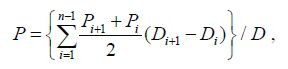 (1)
(1)where P is the mean value of the water column Chl a concentration, Piis the Chl a concentration at layer i, D is the maximumsampling depth, Diis the depth at layer i, and n is the numberof sampling layers.The calculationexpre ssed above is referred to as the depth-weighted value, assuming homogeneity within the water columnother than the depth-integrated value (column burden) .
All contour maps were createdusing Surfer 10 program (GoldenSoftware, Inc) and Ocean Data View 4.5 (ODV) software (Schlitzer, 2010) . Color scatter diagramsand linear regressions were processed by OriginPro 8.5.0 software. Temporal and spatial fluctuations in depth and diel data, and sizefractionated Chl a were tested statistically using parametric or nonparametric tests on the analysis of variance (SPSS 19.0 software) .
3 RESULT AND DISCUSSION 3.1 Environmental factorsWater column temperature and salinity, recorded from August to September2014, varied from 14.25-29.95 (22.43±5.02) ℃ and 23.62-34.61 (34.15±0.66) , respectively. The mean sea surface temperature and salinity were 29.49±0.55℃ and 33.08±0.86, respectively. Verticalprofiles of temperature suggested that the water column was well stratified throughout the entire sampling area. Vertically homogeneous high salinity occupiedall stations, with the exceptionof station A9, where temperature was high and salinity was low (Fig. 2) . The water column at SEATS and adjacent regions had high temperature and high salinity (Figs. 3, 4) . The mean salinity of coastal (<200 m) and pelagic water (>200 m) was 33.77 and 34.24, respectively (Fig. 4) . At the two time-series stations of SEATS (Fig. 5a and c) and J4 (Fig. 5c and d) , the vertical distribution of temperature and salinityin the seawater column was temporally stable.

|
| Figure 2 Transectional distribution of temperature and salinity in the euphotic zone (<200 m) |

|
| Figure 3 Temperature and salinity in the NSCS water layers shallower than 200 m |

|
| Figure 4 Coupled diagramsbetween temperature and salinity in coastal and pelagic regimes |

|
| Figure 5 Verticaldistributions of temperature and salinity at the two time-series stations |
Total Chl a concentrations ranged from 0.006 to 1.488 μg/L, with an average of 0.259±0.247 μg/L. The lowest Chl a concentration was observedin the 200 m water layer at station K2 and the highest in the surface layer of stationA9, which was closest to the Zhujiang River discharge (Fig. 6a) .The Chl a concentration in the coastal domain was much higher than in the offshore area. The depth-weighted Chl a concentration varied between 0.145 and 1.007 μg/L (0.321±0.250 μg/L) . The contributions of various Chl a fractions was shown in Fig. 6a, b. It was observed that the percentagecontribution of picoplankton was higher in deep basin waters than in shallow waters. During periods of low Chl a biomass, a higher proportion of the pico fractionwas observed (Iriarte and Purdie, 1994) . Chl a was generallyhigher in shallow water (<200 m) than in deep water (>200m) , with mean values of 0.364±0.311 μg/L and 0.206±0.192 μg/L, respectively. In our study, examining the size-fractioned Chl a indicated that the contribution of picoplankton to total Chl a biomass, both for the surface layer (Fig. 6a) and the depth-weighted water column (Fig. 6b) , increased from the coastal area to the pelagicregions. This is probablycaused by the variable nutrient concentrations in different regions:the macronutrient concentrations (such as nitrate and phosphate, see Fig. 6c) were, in general, lower in the offshore areas compared to the coastal waters. Owing to their small size, picoplankton has an advantage over other phytoplankton groups in nutrient absorption dynamics in oligotrophic waters (Jiao and Ni, 1997) ; this would, therefore, explainthe relatively higher average percentage of picoplankton Chl a in the deep-water basins (>200 m) than that of shallow (<200 m) waters (Fig. 7) . Except for at stationA9, the total Chl a biomass peaked in the subsurface layer (30-50 m) (Fig. 8a) . In the present study, the Deep Chlorophyll Maximum (DCM) was located at 50-75 m in the SCS, with homogenous concentrations between 100-200 m (Fig. 8) .

|
| Figure 6 Size-fractionated Chl a contributions to total Chl a biomass and nutrient composition |

|
| Figure 7 Size-fractionated Chl a contributions to total Chl a biomass (as percentages of depth-weighted data) in (a) shallow (<200 m) and (b) deep basin (>200 m) waters |

|
| Figure 8 Vertical profiles of Chl a (μg/L) , phaeopigment (μg/L) and the phaeopigment/Chl a ratio in the survey area |
Phaeopigment values (Fig. 8e) ranged from 0.007 to 0.572 (0.127±0.164 μg/L) and the depth-weighted value was 0.111-0.453 (0.127±0.157 μg/L) . Phaeopigment showed increasing from the offshore area to the nearshorearea. Phytoplankton and zooplankton were highly abundant, due to eutrophication resulting from the ZhujiangRiver plume. Strong grazingactivity induces numerous degradation products, typically phaeopigment (Suzuki and Fujita, 1986; Fundel et al., 1998) .
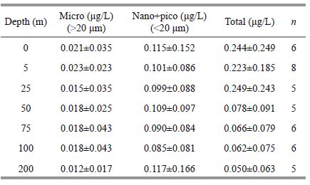
3.2.2 Size-fractionated Chl aThe maximal Chl a concentrations of all size classes were observedin the inshore area, exceptfor picoplankton (Fig. 8) . In addition, the nano-class showed higher values at water depths of 25 m and 50 mat station J3 and 50 m at station J4 (0.365, 0.344, 0.363 μg/L) , but lower than depthof 0 m at station A9 (1.149 μg/L) (Fig. 8c) . Relatively higher valuesof the pico-class were observedat station J3, J4 and J5, compared with those in the neighboring waters (Fig. 8b) . The highestconcentration of pico-class Chl a (0.287 μg/L) was found at ~50 m water depth at station J5. Table 1 shows the value of size-fractionated Chl a at each samplingdepth. A comparison among size fractions showed clearly that the <20-μmfraction (nano-plus pico-plankton) accounted for a larger proportion of overall Chl a than any other size class of Chl a, throughout the entire periodof study.
|
There was a significant difference (Kruskal-Wallis test; P<0.05) in Chl a fractions among the three group depths (Table 2) . The sevendepth data was compiled into three groups based on vertical temperature pattern (Fig. 2) ;the upper mixed layer (0-50 m) , DCM (75 m) and bottomlayer (100-200 m) .

|
Two time-series stations were investigated to understandthe diurnal fluctuations in phytoplankton biomass, by measuring the size-fractionated Chl a concentrations. Diurnal variation in phytoplanktonChl a biomass was observedat both stations, but were not significantly different (One-way ANOVA, α=0.05) .
3.3.1 Total Chl aTime-series observations were conducted at 6-hour intervals over 3 days at station SEATS (Fig. 9a-d) , and at 12-hourintervals over 3 days at station J4 (Fig. 9c-h) . The average Chl a biomass at stations SEATS and J4 was 0.232±0.181 and 0.307±0.179 μg/L, respectively. At station SEATS, the total Chl a concentration was generally higher at 75 m, than in other water layers. At station J4, the maximumtotal Chl a concentration was observedat a water depth of 50 m. Irradiance, temperature, nutrient uptake and carbonassimilation were the factors most likely to be controlling the distribution of the Chl a maxima, based on previous studies (Shimada, 1958; Goering et al., 1964; Yentsch and Ryther, 2003) . In Yentsch and Ryther (2003) , a Chl a maxima occurred in the morning and afternoon, and decreased at midday and atnight. In our study, there were two peaks, at water depths of 75 m at 14:00 and 12:00 at stationSEATS, mainly composedof picoplankton biomass.Similarly, Ning et al. (2004) concluded that phytoplankton biomass was primarily comprised of picoplankton in the SCS area. One peak occurredat 50 m at stationJ4 at 14:00. In the present study, the total phytoplankton Chl a biomass reached a maximum duringthe daytime. Thisis consistent with the hypothesis that phytoplankton tends to propagate in the daytime to make good use of the sunlight, furthermore, the dynamics of Chl a biomass are probablyaffected by zooplankton grazingand diurnal verticalmigration of phytoplankton (Tang and Chen, 2006) .

|
| Figure 9 Temporal distribution of Chl a (μg/L) at mooring stations (SEATS & J4) |
Temporal variations in the contribution of each fraction to the phytoplankton biomass is shownin Fig. 9. The pico-size fraction at station SEATS peaked in the daytime at 08:00, 14:00 and 06:00 with amaximum value of 0.476 μg/L, and then decreasedat dusk (Fig. 9b) . At station SEATS, variations in the nano-size fractionwere similar to the pico-size fraction. In these waters, the micro-size has the smallest averagecontribution (5.95±7.32%) . The phytoplankton biomass was dominatedby the pico-and nano-fraction. Theirproportions are larger in more oligotrophic waters (Polat and Aka, 2007) . At station J4, the mean level of nano-size fractionChl a concentrationwas highest across all size fractions. The highest concentrations of nano- (0.573 μg/ L, Fig. 9g) and micro- (0.072 μg/L, Fig. 9h) size Chl a at station J4 were both found at 14:00, with an opposite pattern observedin the pico-size fraction. A high value of pico-size Chl a was found at 02:00, when the light level was low.
The reduced contribution of picoplankton Chl a to the total Chl a biomass at stationJ4 was owing to its relatively high nutrient concentrations, compared with offshore station SEATS (Agawin et al., 2000) .
3.4 Effectof environmentalfactors on Chl aTemperature, salinityand nutrient availability may play key roles in regulating spatial-temporal shifts between different sizedfractions of Chl a biomass in the Zhujiang River estuary. However, the effects of individual environmental factors cannot be statistically separated (Agawin et al., 2000; Qiu et al., 2010) .
Nutrient distribution in the surface layer at all stations is shown in Fig. 6c. Relatively low concentrations were observedat the oceanic stations. However, patterns in the depth-weighted value of nutrient concentrations differed (Fig. 6d) , with less differencesobserved between coastaland offshore stations. Relationships between synchronized nutrient mapping data and fractionated Chl a compositions are shown in Fig. 10. Significantnegative correlations were observedbetween pico-Chl a and DIN (correlation coeffcient, R2=0.33) and SiO3-Si (R2=0.22) . Both micro-and nano-Chl a were positively correlated with DIN (micro, R2=0.05; nano R2=0.2) and SiO3-Si (micro, R2=0.02; nano R2=0.24) . Phosphorus (P) values made no clear impact on all size fractionsof Chl a (R2=0.001-0.005) , as P limitation was more locally (Sohm and Capone, 2006) . Phosphorus in the oceanprimarily comes from river runoff (Baturin, 2003) , and thus phosphate concentration is likely to be limitedin oligotrophic tropical waters. Comparative studies on the inner shelf and offshorearea have shown that picoplankton has the opportunity to outgrow other size fractionsin areas of high salinity and transmittance, with an affnity for low nutrientconcentrations (Wawrik et al., 2003; Wang et al., 2014) .

|
| Figure 10 Relationships between fractionated chlorophyll a percent and nutrientmapping data at all water depths |
It is suggestedthat seawater deliveredfrom the South China Sea water with high temperature and highsalinity in the Luzon Straitand Kuroshio water has profoundeffects on the adjacentoffshore realm, leading to low phytoplankton abundance (Tan et al., 2013) . However, in the present study, the relatively large influence of the Zhujiang River plume mainly affects the structure and abundance of Chl a fractions in near shore stations. Thus, these two contrasting regions may be characterized by different biogeographic features.
Based on the distribution of phaeopigment in Fig. 8e, we observed that phaeopigment concentrations tended to decrease offshore, with the exceptionof a lesser maxima at station SEATS. The vertical profile of phaeopigment was in parallelto total Chl a. The ratio of Phaeo to Chl a (Fig. 8f) was highest at the 75 m water depth at stationJ5, suggesting phytoplankton death and settlement were more active here. Apart from the coastal stations influencedby the Zhujiang River discharge, phaeopigment contributes more to total Chl a at greater depths.It can be speculated that the conversion between phaeopigment and Chl a in the investigated region is mainly affected by lightintensity and nutrientconditions. This might also imply higher grazingrates by zooplankton at these depths.
4 CONCLUSIONThis study presentssome important information to help understand the distribution and diurnal dynamics of the total and size-fractionated Chl a biomass in the NSCS. The mean totalChl a and phaeopigment concentrations in the investigated areas were 0.259±0.247 and 0.127±0.164 μg/L, respectively. The comparative study in coastal and offshore areas revealed apparent heterogeneity. Vertically, the maximum value appearedat depths of 30-50 m, and statistical analysis suggested significant vertical variations in Chl a biomass. In the study area, picoplankton and nanoplankton were the major components of the total Chl a biomass. The size-fractionated Chl a exhibited linear correlations with nutrient concentrations. In addition, differential diurnal dynamics of total Chl a biomass and different Chl a size classes were observed in the two contrasting environments (coastal and oceanic area) , which has not been reported in previously studies. The information presentedhere helps us better understand the spatialand temporal patternsin size-fractionated Chl a biomass in different regions of the NSCS and theirmajor environmental controlling factors. This study will also contribute to our understanding of phytoplanktoncommunity structure and the environmental factorsregulating the distribution of different phytoplankton functional groups in the NSCS.
5 ACKNOWLEDGEMENTThe authors would like to thank WEI Yuqiu, LI Zhuo and SHU Yi, as well as the captain and crew of R/V Shiyanyi for their assistanceduring the summer cruise. We thank Dr. CHEN Songze and his workmate from Tongji University for field nutrient seawater sampling. The synchronized nutrientdata, provided by Dr. SUN Jia from Xiamen University, was also appreciated. Commentsand suggestions from the editor, Professor Doug Campbell and two anonymous reviewers strengthened the manuscript.
| Agawin N S R, Duarte C M, Agustí S, 2000. Nutrient and temperature control of the contribution of picoplankton to phytoplankton biomass and production. Limnol. Oceanogr., 45 (3) : 591 –600. Doi: 10.4319/lo.2000.45.3.0591 |
| Azov Y, 1991. Eastern Mediterranean-a marine desert? Mar. Poll. Bull., 23 : 225 –232. Doi: 10.1016/0025-326X(91)90679-M |
| Baturin G N, 2003. Phosphorus cycle in the ocean. L ithol. Miner. Resour., 38 (2) : 101 –119. Doi: 10.1023/A:1023499908601 |
| Berman T, Azov Y, Schneller A, Walline P, Townsend D W, 1986. Extent, transparency and phytoplankton distribution of the neritic waters overlying the Israeli coastal shelf. Oceanol. Acta, 9 (4) : 439 –447. |
| Bianchi T S, Findlay S, Fontvieille D, 1991. Experimental degradation of plant materials in Hudson river sediments. Biogeochemistry, 12 (3) : 171 –187. |
| Che H, Ran X B, Zang J Y, Liu J, Zheng L, Qiao F L, Zhan R, 2012. Distributions of size-fractions of Chlorophyll a and its controlling factors in summer in the southern South China Sea. J. Hydroecol., 33 (4) : 63 –72. |
| Chen C C, Kwo S F, Chung S W, Liu K K, 2006. Winter phytoplankton blooms in the shallow mixed layer of the South China Sea enhanced by upwelling. J. Mar. Syst., 59 (1-2) : 97 –110. Doi: 10.1016/j.jmarsys.2005.09.002 |
| Fundel B, Stich H B, Schmid H, Maier G, 1998. Can phaeopigments be used as markers for Daphnia grazing in Lake Constance? J. Plankton Res., 20 (8) : 1449 –1462. Doi: 10.1093/plankt/20.8.1449 |
| Gieskes W W C, Kraay G W, Baars M A, 1979. Current 14 C methods for measuring primary production: gross underestimates in oceanic waters. Neth. J. Sea Res., 13 (1) : 58 –78. Doi: 10.1016/0077-7579(79)90033-4 |
| Goering J J, Dugdale R C, Menzel D W, 1964. Cyclic diurnal variations in the uptake of ammonia and nitrate by photosynthetic organisms in the Sargasso Sea. Limnol. Oceanogr., 9 (3) : 448 –451. Doi: 10.4319/lo.1964.9.3.0448 |
| Gong G C, Liu K K, Liu C T, Pai S C, 1992. The chemical hydrography of the South China Sea west of Luzon and a comparison with the West Philippine Sea. Terrestrial. Atmos. Ocean Sci., 3 (4) : 587 –602. |
| Guo Y J, Ye J S, Zhou H Q, 1978. Quantitative distribution of phytoplankton in Xisha & Zhongsha Islands. Beijing: Science Press1-10. |
| Helling G R, Baars M A, 1985. Changes of the concentrations of chlorophyll and phaeopigment in grazing experiments. H ydrobiol. B ull., 19 (1) : 41 –48. |
| Ho A Y T, Xu J, Yin K D, Jiang Y L, Yuan X C, He L, Anderson D M, Lee J H W, Harrison P J, 2010. Phytoplankton biomass and production in subtropical Hong Kong waters: influence of the Pearl River outflow. Estua r. Coast, 33 (1) : 170 –181. Doi: 10.1007/s12237-009-9247-8 |
| Hu Z F, Tan Y H, Song X Y, Zhou L B, Lian X P, Huang L M, He Y H, 2014. Influence of mesoscale eddies on primary production in the South China Sea during spring intermonsoon period. Acta Oceanol. Sin., 33 (3) : 118 –128. Doi: 10.1007/s13131-014-0431-8 |
| Iriarte A, Purdie D A, 1994. Distribution of chroococcoid cyanobacteria and size fractionated chlorophyll a biomass in the central and southern North Sea waters during June/ July 1989. Neth. J. Sea Res., 31 (1) : 53 –56. |
| Jeffrey S W. 1980. Algal pigment systems. In: Falkowski P G ed. Primary Productivity in the Sea. Plenum Press, New York. p.35-38. |
| Jiao N Z, Ni I H, 1997. Spatial variations of size-fractionated chlorophyll, cyanobacteria and heterotrophic bacteria in the Central and Western Pacific. H ydrobiologia, 352 (1-3) : 219 –230. |
| Le F F, Ning X R, 2006. Variations of the phytoplankton biomass in the northern South China Sea. J. Mar. Sci., 24 (2) : 60 –69. |
| Le F F, Ning X R, Liu C G, Hao Q, Cai Y M, 2008. Standing stock and production of phytoplankton in the northern South China Sea during winter of 2006. Acta Ecol. Sin., 28 (11) : 5775 –5784. |
| Le F F, Sun J, Ning X R, Song S Q, Cai Y M, Liu C G, 2006. Phytoplankton in the northern South China Sea in summer 2004. Oceanol. Limnol. Sin., 37 (3) : 238 –248. |
| Li K Z, Guo Y J, Yin J Q, Huang L M, 2005. Phytoplankton diversity and abundance in Nansha islands waters in autumn of 1997. J. Trop. Oceanogr., 24 (3) : 25 –30. |
| Li T, Liu S, Huang L M, Zhang J L, Yin J Q, Sun L H, 2008. Studies on a Trichodesmium erythraeum red tide in Daya Bay. Mar. Environ. Sc i., 27 (3) : 224 –227. |
| Lin I I, Lien C C, Wu C R, Wong G T F, Huang C W, Chiang T L, 2010. Enhanced primary production in the oligotrophic South China Sea by eddy injection in spring. Geophys. Re s. Lett., 37 (16) : L16602 . |
| Liu Z L, Ning X R, Cai Y M, 1998. Distribution characteristics of size-fractionated chlorophyll a and productivity of phytoplankton in the Beibu Gulf. Acta Oceanol. Sin., 20 (1) : 50 –57. |
| Lorenzen C J, Welschmeyer N A, Copping A E, 1983. Particulate organic carbon flux in the subarctic Pacific. Deep Sea Res., 30 (6) : 639 –643. Doi: 10.1016/0198-0149(83)90041-9 |
| Ma W, Sun J, 2014. Characteristics of phytoplankton community in the northern South China Sea in summer and winter. Acta Ecol. Sin., 34 (3) : 621 –632. |
| Ning X, Chai F, Xue H, Cai Y, Liu C, Shi J, 2004. Physicalbiological oceanographic coupling influencing phytoplankton and primary production in the South China Sea. J. Geophys. Res., 109 (C10) : C10005 . Doi: 10.1029/2004JC002365 |
| Odate T, Maita Y, 1989. Regional variation in the size composition of phytoplankton communities in the western North Pacific ocean, spring 1985. Biol. Oceanogr., 6 (1) : 65 –77. |
| Parsons T R, Maita Y, Lalli C M. 1984. A Manual of Chemical and Biological Methods for Seawater Analysis. Pergamin Press, Oxford. p.173. |
| Peng X, Ning X R, Sun J, Le F F, 2006. Responses of phytoplankton growth on nutrient enrichments in the northern South China Sea. Acta Ecol. Sin., 26 (12) : 3959 –3968. |
| Platt T, Subba Rao D V, Irwin B, 1983. Photosynthesis of picoplankton in the oligotrophic ocean. Nature, 301 (5902) : 702 –704. Doi: 10.1038/301702a0 |
| Polat S, Aka A. 2007. Total and size fractionated phytoplankton biomass offKaratas, north-eastern Mediterranean coast of Turkey. J ournal Black Sea / Mediterranean Environment, 13: 191-202. |
| Qiu D J, Huang L M, Zhang J L, Lin S J, 2010. Phytoplankton dynamics in and near the highly eutrophic Pearl River Estuary, South China Sea. Cont. Shelf Res., 30 (2) : 177 –186. Doi: 10.1016/j.csr.2009.10.015 |
| Schlitzer R. 2010. Ocean data view. http://odv.awi.de2010. |
| Shen P P, Tan Y H, Huang L M, Zhang J L, Yin J Q, 2010. Occurrence of brackish water phytoplankton species at a closed coral reef in Nansha Islands, South China Sea. Mar. Pollut. Bull., 60 (10) : 1718 –1725. Doi: 10.1016/j.marpolbul.2010.06.028 |
| Shimada B M, 1958. Diurnal fluctuation in photosynthetic rate and chlorophyll a content of phytoplankton from Eastern Pacific Waters. Limnol. Oceanogr., 3 (3) : 336 –339. Doi: 10.4319/lo.1958.3.3.0336 |
| Sohm J A, Capone D G, 2006. Phosphorus dynamics of the tropical and subtropical north Atlantic: Trichodesmium spp. versus bulk plankton. Mar. Ecol. Prog. Ser., 317 : 21 –28. Doi: 10.3354/meps317021 |
| Song X Y, Huang L M, Qian S B, Yin J Q, 2002. Phytoplankton diversity in waters around Nansha Islands in spring and summer. Biodivers. Sci., 10 (3) : 258 –268. |
| Su J L, 2005. Overview of the South China Sea circulation and its dynamics. Acta Oceanol. Sin., 27 (6) : 1 –8. |
| Sun J, Song S Q, Le F F, Wang D, Dai M H, Ning X R, 2007. Phytoplankton in the northern South China Sea in winter of 2004. Acta Oceanol. Sin., 29 (5) : 132 –145. |
| Suzuki R, Fujita Y, 1986. Chlorophyll decomposition in Skeletonema costatum: a problem in chlorophyll determination of water samples. M ar. Ecol. Prog. Ser., 28 : 81 –85. Doi: 10.3354/meps028081 |
| Tan J Y, Huang L M, Tan Y H, Lian X P, Hu Z F, 2013. The influences of water-mass on phytoplankton community structure in the Luzon strait. Acta Oceanol. Sin., 35 (6) : 178 –189. |
| Tang S M, Chen X Q, 2006. Phytoplankton diel rhythm in the waters of Quanzhou Bay in Fujian, China. Acta Oceanol. Sin., 28 (4) : 129 –137. |
| Wang B L, Liu C Q, Wang F S, Li S L, Patra S, 2014. Distributions of picophytoplankton and phytoplankton pigments along a salinity gradient in the Changjiang River Estuary, China. J. Ocean U niv. China, 13 (4) : 621 –627. Doi: 10.1007/s11802-014-2362-6 |
| Wang Z H, Qi Y Z, Chen J F, Xu N, Yang Y F, 2006. Phytoplankton abundance, community structure and nutrients in cultural areas of Daya Bay, South China Sea. J. Mar. Syst., 62 (1-2) : 85 –94. Doi: 10.1016/j.jmarsys.2006.04.008 |
| Wang Z H, Zhao J G, Zhang Y J, Cao Y, 2009. Phytoplankton community structure and environmental parameters in aquaculture areas of Daya Bay, South China Sea. J. Environ. Sci., 21 (9) : 1268 –1275. Doi: 10.1016/S1001-0742(08)62414-6 |
| Wawrik B, Paul J H, Campbell L, Griffi n D, Houchin L, Fuentes-Ortega A, Muller-Karger F, 2003. Vertical structure of the phytoplankton community associated with a coastal plume in the Gulf of Mexico. Mar. Ecol. Prog. Ser., 251 : 87 –101. Doi: 10.3354/meps251087 |
| Ye J S, Lin Y S, Yuan W B, 1983. Quantitative distribution of phytoplankton in the East Sand Island sea area in summer. Beijing: Ocean Press, Beijing, China1-6. |
| Yentsch C S, Ryther J H, 2003. Short-term variations in phytoplankton chlorophyll and their significance. Limnol. Oceanogr., 2 (2) : 140 –142. |
| Zhang T H, Zhan H G, Chen C Q, 2007. Analyses on spatial variation of chlorophyll in surface layer of South China Sea. J. Trop. Oceanogr., 26 (5) : 9 –14. |
| Zhao H, Qi Y Q, Wang D X, Wang W Z, 2005. Study on the features of chlorophyll-a derived from SeaWifs in the South China Sea. Acta Oceanol. Sin., 27 (4) : 45 –52. |
| Zhao J, Yao P, Yu Z G, 2010. Progress in marine sedimentary pigments as biomarkers. A dvances in Earth Science, 25 (9) : 950 –959. |
| Zhou W H, Yuan X C, Huo W Y, Yin K D, 2004. Distribution of chlorophyll a and primary productivity in the adjacent sea area of Changjiang River Estuary. Acta Oceanol. Sin., 26 (3) : 143 –150. |