 2016, 34
Institute of Oceanology, Chinese Academy of Sciences
Article Information
- Xingjie JIANG(江兴杰), Daolong WANG(王道龙), Dalu GAO(高大鲁), Tingting ZHANG(张婷婷)
- Experiments on exactly computing non-linear energy transfer rate in MASNUM-WAM
- Journal of Oceanology and Limnology, 34(4): 821-834
- http://dx.doi.org/10.1007/s00343-016-5007-3
Article History
- Received: Jan. 8, 2015
- Accepted: Jan. 5, 2016


2. First Institute of Oceanography, State Oceanic Administration, Qingdao 266061, China
It is nowadays widely accepted that weak-resonance non-linear energy transfer between sea waves plays a very important role in energy dispersion. The theoretical framework of the wave-wave nonlinear interaction was developed in the 1960s(Hasselmann, 1962, 1963a). A 6-fold Boltzmann integral was formulated to describe these non-linear interactions and many researchers spent much effort developing various schemes to compute the integral on computers(1963b; Webb, 1978; Masuda, 1980). Termed exact computations or full Boltzmann integral(FBI), these schemes considered all resonance configurations.
Because of their complexity and time demands, these exact methods are not suitable for inclusion in operational spectral wave models. Various approximate methods have been developed to improve the computational efficiency(Barnett, 1968; Ewing, 1971; Hasselmann and Hasselmann, 1981). Finally, the discrete interaction approximation(DIA) (Hasselmann and Hasselmann, 1985a; Hasselmann et al., 1985)was widely accepted and triggered the development of the third-generation wave models, like WAM(The Wamdi Group, 1988), the WaveWatch (Tolman, 1991)and the SWAN model(Booij et al., 1999). The DIA is much more efficient than exact computations because it considers only one pair of resonance configurations. The DIA preserves a few but important characteristics of the full solution, such as the slow downshifting of the peak frequency and the shape stabilization during wave growth.
Nevertheless, the DIA also shows some deficiencies, such as allocating too much energy from the spectral region near the spectral peak to higher frequencies(van Vledder et al., 2000). The known deficiencies of the DIA in a prediction model will not infl uence bulk wave parameters, such as the significant wave height, the zero-crossing period, and the mean wave direction, but it does distort the shape of energy spectra, which are vital in research on waves.Therefore, it is preferable to include an exact computation or FBI in a wave model for purposes of research. There are some third-generation wave models that have included exact computations, such as WaveWatchIII(Tolman, 2002), SWAN(Booij et al., 2004), CREST(Ardhuin et al., 2001), and PROWAM(Monbaliu et al., 1999).
The performance of exact computations has been well understood(Hasselmann and Hasselmann,1985c; van Vledder, 2006), but the effects of such methods in a certain wave model still need to be studied individually. In this paper, we describe the implementation of the Webb-Resio-Tracy(WRT) method(Webb, 1978; Tracy and Resio, 1982; Resio and Perrie, 1991)into MASNUM(the Key Laboratory of Marine Science and Numerical Modeling, First Institute of Oceanography, SOA, China)wave model (Yuan et al., 1992a, b; Yang et al., 2005). MASNUMWAM is a third-generation model which calculates energy spectrum balance equation using a characteristics inlaid scheme; the dissipation source function of this model is based on the wave broken statistic theory(Yuan et al., 1986); MASNUM-WAM adopts wave number spectral space which is coherent with the wave-wave nonlinear interaction theory (Hasselmann, 1962, 1963a). The WRT programs we used are free software distributed by Gerbrant Ph. van Vledder, ALKYON Hydraulic Consultancy & Research; the latest version is 5.04. In Section 2, we briefl y introduce the theoretical background of the WRT method, the modifications we made and numerical procedures we developed. In Section 3, we describe a series of numerical experiments to illustrate the ease and efficiency of the implementation. Finally, in the last section, we discuss current and future work.
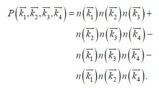
2 THEORETICAL BACKGROUND AND METHODS 2.1 Theoretical background 2.1.1 The WRT methodThe WRT method is widely accepted as a mature and stable exact-computation scheme for non-linear energy transfer. Following Hasselmann(1962), the original 6-fold Boltzmann integral is
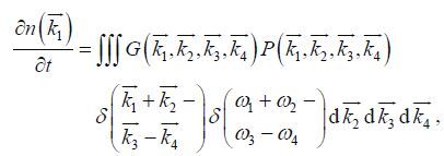 (1)
(1)where 

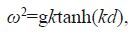 (2)
(2)in which g is the acceleration of gravity and d local depth. The wave number and frequency resonance condition
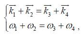 (3)
(3)
are contained in the two delta-functions of the integral. The coupling coefficient G is a complicated function of wave numbers and frequencies, and 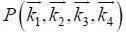
 (4)
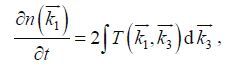
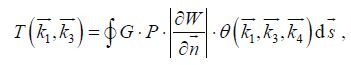
(4) A key aspect in the WRT method is to consider the integration space for each 
 (5)
(5)where
 (6)
(6)with 
 (7)
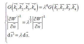
(7)The above summarizes the basic theory of Webb (1978); additional work has been done by Tracy and Resio(1982)and Resio and Perrie(1991).
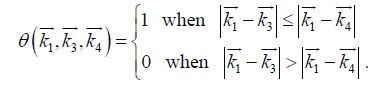
2.1.2 Geometric scalingFor convenience, we use a geometric scaling spectral space, in which k i +1 = λk i with λ > 1. Such scaling provides a higher spectral resolution near the peak of the spectrum and less resolution in the highfrequency tail. An optimization algorithm was developed based on the geometric spacing spectral grid(Tracy and Resio, 1982). In the geometrical scaling k -space, if 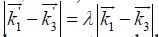


 (8)
(8)Therefore, with some basic pairs of $\overrightarrow {{k_1}} $ and $\overrightarrow {{k_3}} $ , a table of all possible values for

Nevertheless, the geometric scaling can only be used when the dispersion relation ω 2 =g k is adopted. Because the coupling coefficient and locus solutions are all based on wave numbers, the Jacobian term, in which W = ω 1 + ω 2 – ω 3 – ω 4 is related to the angular frequency. Geometrical spacing is not allowed in both wave-number space and angular-frequency space in Eq.2 where a finite water depth is considered. Mismatching in the geometrical spacing may lead to incorrect results in Eq.8 and W =0 is the basic resonance condition that cannot be avoided by any scheme.
2.1.3 Pre-calculation and grid-searchingAnother important property of the WRT method is that all of the loci, interpolation coefficients, coupling coefficients, and Jacobian terms are only associated with the(wave number)spectral grid and water depth, but have nothing to do with the shape of the spectrum. For a given discrete spectral grid and water depth, all of those parameters mentioned above can be precomputed and stored in memory or in a database on disks, and then a search-and-read process could be performed instead of a repeated calculation if the current spectral grid and depth match.
The grid-searching technique is based on some pre-calculated depths. New computations for the local depth are avoided, and the program tries to find a nearest pre-calculated depth record instead. The final results will then be scaled by a factor based on the local and nearest depths. More details can be found in Section 2.3.
2.2 Modifications 2.2.1 Spectral space transformationIn the originally distributed WRT subroutines, the angular-frequency spectral space(ω -space)is adopted, which is also adopted in WaveWatchIII and SWAN models. However, as we have seen in Section 2.1, the core integral processes are all based on the wave number spectral space(k -space). The action density terms can be transformed between ω -space and k -space following
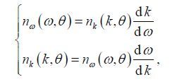 (9)
(9)with the dispersion relation Eq.2.
For wave models like WaveWatchIII and SWAN, it may be convenient to interact with the outside main program with ω -space. However, once the ω -space is set in the main program and fixed during the whole computation, the k -space needs to be reinitialized according to Eq.9 every time when the WRT computation takes place at a geographic grid where a new depth d is met, which seems necessary but time consuming. Another disadvantage of frequent reinitialization is that the pre-calculation technique is not well exploited, because all of the pre-calculated parameters are dependent on the core k -space, and once the k-space is changed, those pre-calculated values will no longer match and hence become useless.
Thus, we transformed the whole WRT scheme into the k-space including introducing a fixed wave number spectral grid that is independent of the original, transforming all spectral related variables into the new spectral space and simplifying some spectral grid checking processes, which is unnecessary now because the spectral space and related parameters will not be changed any more during the whole computation. However, the variables of the group speed, which depend on local depth, still need to be revalued for each grid.f
As mentioned above, wave spectra in MASNUMWAM are also solved in a wave number space. After the transformation, the interaction between the main program and the WRT subroutines are more convenient now. We adopt the same spectral space used in the main program and the initialization is performed only once at the initializing part of the model. The pre-calculated records also can be accessed more efficiently now. More details are given in Section 2.3.
2.2.2 Parallel computationParallel computing is a useful technique to improve computation speed, and MASNUM-WAM supports the MPI Parallelization(Wang et al., 2007). In the MPI version of MASNUM-WAM, each CPU is assigned to a part of the modeling sea area and each CPU process has its own independent task, except data communicated on boundaries. When the original WRT method is parallelizing, each CPU manages its own memory but accesses files on the disk only according to filenames, such as error files, log files, and also pre-computed files. If two or more CPUs access the same file at the same time, the whole computation job stops. To solve this problem, we added CPU ids in all of the filenames stored on the disk allowing each CPU use its own files without interference. Those modifications made it possible to perform large-scale computation for real case modeling.
2.3 Numerical procedures designThe original WRT subroutines can be separated into two kinds of functions, those that initialize the configurations and those that execute the main computation. They also provide some acceleration techniques such as geometric scaling, the precalculation, and grid-searching techniques. To produce better computational efficiency, these functions and techniques need to be well reorganized and optimized under the computation structure of the implemented model. Thus, we developed four numerical procedures which can implement the basic functions and use the acceleration techniques in the best possible way. Furthermore, the spectral space transformation mentioned above may give rise to additional efficiencies. Experiments described in Section 3 will verify efficacy and compare procedure efficiencies.
The four numerical procedures are denoted NP1, NP2, NP3 and NP4, and outlined in Fig. 1a–d. NP1 is designed for infinite depth whereas the other three are for finite depth. Each of the procedures has an initial part and a main part, both of which will access the memory or the disks for data reading and writing. The initial parts are similar in that the basic configurations of the WRT scheme are set and the loci-related grids and coefficients are prepared for one or several depths. Because of a fixed spectral space has been adopted, the initial part needs to be executed only once and most of the spectral grid-related configurations need no revaluation. The main parts, however, are very different and complicated, having to be repeated many times for each time loop and topographical grid.

|
| Figure 1 Flow diagrams of the four numerical procedures |
NP1(Fig. 1a)is designed for deep water. Thus, only max-depth, which is set to 9 999 m, is precalculated and related information is stored in memory. In the main part, all needed data for the main computation can be loaded from memory, which is much faster than looking up from disks. For infinite depth, the dispersion relationship ω 2 =g k is adopted; hence, the geometric scaling technique can be triggered. Efficiency improvements can be found in Section 3.
For finite depth, procedures are more complicated. The NP2 deals with finite-depth situations by way of scaling the infinite results by a factor. Hence, it has the same initial and main part as in NP1, except the non-linear energy transfer rate finally multiplies an observed magnitude scaling factor, which is parameterized with a simple function(Herterich and Hasselmann, 1980; The Wamdi Group, 1988)
 (10)
(10) (11)
(11)where d is the local depth. This method seems easy and fast. Furthermore, the deep-water dispersion relation is still adopted and the geometric scaling also can be enabled.
Different from scaling the final transfer rate in NP2, another option for finite depth is NP3, shown in Fig. 1c, which uses a depth-dependent coupling coefficient(Herterich and Hasselmann, 1980). Differences between the two methods have been discussed in detail based on a JONSWAP spectrum (van Vledder, 2006), but effects of the two options in an operational wave model are still unclear(to be discussed later in Section 3). Because a variety of depths are considered now, more pre-calculations are performed in NP3. In the initial part, only the maxdepth is pre-calculated. However, in the main part, a check on whether a pre-calculated file for current depth exists is performed first. If the file exists, the record will be loaded from the database; if not, a new calculation will be performed and the new record added into the database for checking next time. Because of the spectral space transform and the uniform spectral grid adopted, all the parameters needed in the main computation are only changed with depth(the current effects are not considered in this paper). Once a recorded depth is found, the data can be loaded directly without any further checks.
After the first traversal of all depths, only a loading of an appropriate record needs to be performed in the remaining loops of NP3, but the pre-calculated files are as numerous as the topographical grid points. NP4 offers a less-files solution by adopting a grid-searching technique. The grid searching technique in the original WRT method finds a nearest pre-calculated depth according to the local one, and a scale factor, based on the local and nearest depths, is generated from Eqs.10 and 11 yielding
 (12)
(12)Thus, in the initial part of NP4, more pre-setting depths are pre-calculated. However the more depths are pre-set, the more time is taken in finding the target but the computation time for calculating scale factor cannot be avoided.
3 NUMERICAL EXPERIMENTSome numerical experiments are now described that were performed based on the numerical procedures presented above. All the experiments were run in the C sector of the “Rubik’s Cube” supercomputer, which is supported by the Shanghai Supercomputer Center(SSC), China. The CPUs used in this supercomputer are AMD Barcelona 1.9 GHz, each of which contains 4 processors.
3.1 Idealized experiments 3.1.1 Wave growth in deep waterFor deep-water scenarios, NP1 is adopted. The ST1 experiments are duration-limited, which consider a steady wind blowing over an unlimited ocean for time t with a reasonable initial condition. Unlimited ocean means the advection terms in the energy balance equation are switched offand only one single grid point is relevant. The time-evolving spectra are all recorded for further study. The ST2 experiment is fetch-limited meaning that it considers a wave propagating along a 1-D space and driven by a uniform and steady wind. The time evolution of the total spectral energy along the 1-D fetch is also recorded.
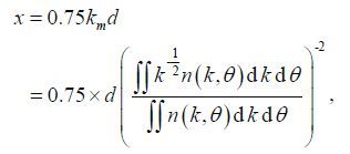
The source terms used in the ST1 and ST2 experiments are the wind input, the wave breaking dissipation, and the nonlinear energy transfer. The simulation time lasts for 300 hours to ensure the wind waves are fully developed in each experiment. The spectral space is set to 40 grids in the k -direction and 36 in the θ -direction. The wave number starts at 0.007 1 rad/m, corresponding to about 0.04 Hz in deep water, and increases by the geometric factor of 1.21. The experiments marked with g s are added to check the efficiency improvement of the geometric scaling technique(the spectral space can be always geometric spaced but the geometric scaling technique is an option to be enabled).
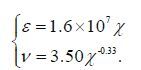
There are five wind speeds(5, 10, 20, 30, 40 m/s) employed to drive the model to examine the consistency; the dimensionless parameters are used for further comparison. The dimensionless spectrum energy is ε=σ2 g2/U 104 , in which σ2 is the wave height variance, i.e., the zero-order moment of the spectrum m 0 and U 10 is the wind speed at a 10-m height above the sea surface. Similarly, the dimensionless peak frequency is v = f p U 10 /g, dimensionless wind duration ς = t(g/ U 10), and dimensionless fetch χ=x(g/U102)with dimensional f p in Hz, t in seconds, and x in meters.
The simulation results are going compared with observed wave growth curves. The JONSWAP fetchlimited wind growth relation(Hasselmann et al., 1980)is
 (13)
(13)Another denoted Donelan85(Donelan et al., 1985)
 (14)
(14)Hwang and Wang(2004), during the propagation of the wave energy, functions of time and space are related by
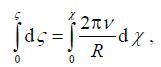 (15)
(15)where R is equal to 0.4 for wind sea. The dimensionless duration and fetch coupled through
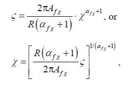 (16)
(16)and the parameters in Eq.16 have fixed values A fχ =11.86, α fχ =-0.236 8.
Figure 2 shows that, with the modified WRT method, the single-grid-point MASNUM-WAM can well simulate the growth of wind-driven sea, because under different steady winds(colored curves)the dimensionless growth produced are similar to the observed results(black curves).

|
| Figure 2 Dimensionless spectral energy and peak frequency growth with dimensionless time |
The fetch-limited experiments are performed in a 1-D spacing model. The waves are assumed to propagate along a 6-degrees(about 667 km)space and computational grid points are set every 0.2 degrees. Figure 3 shows the fully developed dimensionless spectral energy along the 1-D fetch compared with measured data( Hasselmann et al., 1980; Donelan et al., 1985).
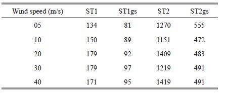
Colored curves in Figs. 2 and 3 are produced when geometric scaling is enabled; Table 1 shows the time taken if geometric scaling is enabled or not. This indicates that geometric scaling can save about 40%–50% of the computation time in these tests.

|
| Figure 3 Dimensionless wave growth with dimensionless fetch depth |
For constant finite depth, NP2 and NP3 are adopted with geometric scaling available in NP2. The performance of the shallow-water schemes in NP2 and NP3 are examined below in a real model.
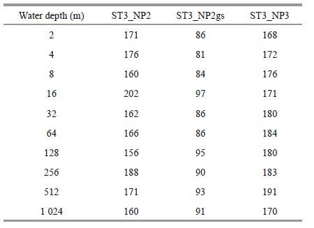
Three groups of tests are made. The ST3_NP2 and ST3_NP3 adopt NP2 and NP3 separately, and ST3_ NP2gs employed the geometric scaling technique. Here, a single-grid-point model like ST1 is employed again, with all the same settings. Tests are performed for different depths, from the very shallow depth of 2m to 1 024 m, which is acceptable as deep water. Figure 4 shows the modeling results, in which we can figure that, effects of the two shallow-water schemes in NP2 and NP3 are indeed different in a real model. However, the differences become small as depth increases to 1 024 m; there is almost no discrepancy. Nevertheless, the continuously growing curves(solid)of ST3_NP3 seem more reasonable. ST3_NP2 and ST3_NP3 take almost the same simulation time, but geometric scaling saves about half of the time without changing the finally effects (dashed and dotted lines in Fig. 4)as indicated in Table 2. Without changes in depth in those tests, the main computation only loads data from memory and no more loci grids are created; hence, a similar time is taken in ST3_NP2 and ST3_NP3.

|
| Figure 4 Dimensionless wave growth in constant depth |
A real scenario of wind waves in deep-water(ST4) is performed with the parallel version of MASNUMWAM. The modeling area is located in the South China Sea with a buoy placed at 115.262 5°E, 19.540 7°N; see Fig. 5(the black triangle). The local water depth is more than 2 100 m and local wind and wave are observed simultaneously.

|
| Figure 5 ST4 modeling area for the South China Sea simulation |
We set the modeling area from 99°E to 125°E, 2°N to 25°N with a resolution of 0.125 degrees, the spectral grid to 35 grid points in the k-direction, beginning with 0.007 1 and geometrically increasing by 1.21, and to 12 grid points in the θ -direction covering a full circle. The driving wind is from the NCEP reanalysis product, which conforms with wind observations of the buoy(Fig. 6). The modeling time is from July 5th to 26th, 2011. During this period, a continuous SSW wind was blowing and the water depth was more than 1 000 m in the SSW direction of the buoy, which can be classified as deep water.

|
| Figure 6 Comparison of wind speed and direction of the NCEP reanalysis product with buoy observations |
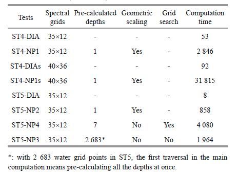
With the DIA method also included, the experiment is denoted ST4-DIA; ST4-NP1 denotes the MPI version of MASNUM-WAM adopting NP1 with geometric scaling enabled. In both computations, we set the same parameters except the non-linear energy transfer source term, and we employed 128 CPUs to run the models. Denoted ST4-DIAs and ST4-NP1s, two additional computations with 40 grids in the k-direction and 36 in the θ -direction as in the idealized experiments are also conducted to compare computation times.
From Fig. 7, ST4-NP1 performs well and proves the viability of such implementations in the parallel version of the wave model. ST4-NP1 performs even better than the DIA method in the mean wave period according to the observation data. However, the computation time for ST4-NP1 is much larger by about 54 times that of the DIA model(Table 3). When the calculated quantity expands about 3 times(ST4- NP1s), the computation time is up to more than 22 days. However, because of the spectral space transform and geometric scaling technique, it is still much smaller than the computation times of 10 3 –10 4 times recorded for WaveWatchIII(Tolman, 2009).

|
| Figure 7 Comparison of simulation results from ST4 with observations |

|
| Figure 8 ST5 modeling area for the Bohai Sea simulation |
The finite-depth real case is denoted as ST5, and the simulation is performed in an area in the Bohai Sea of China. Connected with the Yellow Sea through the Bohai Strait, the Bohai Sea is a closed sea area with a mean depth of about 20 m. A buoy is situated in the Bohai Strait with a depth of 33 m(121.068 0°E, 38.158 5°N), and the wave field of this area is infl uenced mostly by winds coming from the East. The ST5 modeling area is set as 119°–126.5°E, 36.5°–40°N with a resolution of 1/12 degrees. The modeling time is from November 5th to 15 th, 2012. The same spectral grid as in ST4 is adopted. The driven wind field is a hindcasting product of the WRF model and a comparison with observed data shows the viability of such driven wind(Fig. 9). For each computation, 48 CPUs were employed.

|
| Figure 9 Comparison of the WRF numerical hindcasting wind with observational data |
With a finite depth, the situation is a more complicated than deep water. There are four tests taken in ST5. ST5-DIA employs the DIA method which with finite depth adopts the same scale function Eq.10 as in NP2. ST5-NP2 and ST5-NP3 adopt NP2 and NP3 separately, and geometric scaling is enabled in ST5-NP2. For ST5-NP4, the pre-calculated depths are set to 2, 4, 8, 16, 32, 64, and 128 meters, as the max-depth of the modeling area is 88 m.
Figure 10 shows the simulation results of the four tests. The wave direction data marks spinning with the time periodically in Fig. 10 looks very strange. We checked the observational data and contacted the manufacturer of the buoy, and finally confirmed that there was something amiss with the wave direction sensor of the buoy. Despite the irregularity in the mean direction of the observed wave, the other wave parameters observed were still valid. The simulation results of the tests with DIA, NP3 and NP4 were in good agreement, although ST5-NP2 deviated from the other three, especially in the mean wave period simulation. From Table 3, the test with DIA is clearly the most efficient. The computation time for the exact method in these tests were 100 to 500 times more than the DIA method, which is still smaller than the computation times reported for WaveWatchIII (Tolman, 2009).

|
| Figure 10 Comparison of simulating results of ST5 with observational data |
Six groups of 60 experiments were performed. The new numerical procedures were adopted according to the water depth for each of the experiments.
For infinite depth, NP1 with the transformed wave number spectral space works very well, and about 40%–50% of the computation time can be saved with the geometric scaling technique. For modeling of real cases with infinite depth, NP1 with geometric scaling only takes about 50 times more time than the DIA method, which is much less than the runtimes for WaveWatchIII. For finite depth, NP2 provides the best efficiency in the exact procedures but gives different results compare with NP3 in the constant finite-depth test and the DIA, NP3 and NP4 in the real-case test. In the real case test, NP2 with geometric scaling takes about 107 times more time than the DIA method, and the well-designed NP3 takes about 245 times more time without geometric scaling.
NP2 and NP3, adopting different shallow-water schemes separately, do not produce results in agreement with the idealized experiments(Fig. 4). A reasonable explanation for the deviation is that, as for the theoretical analysis(van Vledder, 2006), the scaled scheme, as for NP2, distributes more energy into higher frequencies; otherwise, the scheme using depth-dependent coupling coefficient, as in NP3 and NP4, distributes energy more uniformly. The total energy is conservative for non-linear transfer, but a growth limiter(Hersbach and Janssen, 1999)should be imposed later to ensure numerical stability but also to fl atten the positive lobe of the spectrum in the equilibrium range. The original conservation is then broken, energy is lost and a smaller significant wave height is generated. The deviation of the energy structure in the spectra could also lead to a prediction of larger wave period, as is seen in Figs. 7 and 10.
Comparing NP4 with the original grid-searching technique, the new NP3 takes less time and yields the same simulation results. Unlike the original WRT method adopting fixed angular-frequency spectral space, the wave number spectral space is often changed for the local environment. Based on the spectral space transform, all spectral space-dependent loci grids, coefficient, and Jacobian terms are fixed for a certain depth because the spectral space is fixed. Checks for such a record are always passed and all of the pre-calculated information can be accepted as long as a correct depth is found. Hence, it is feasible to pre-calculate all depths once and then load a particular one directly, even though there are as many pre-stored files as topographical grids. Otherwise the grid-searching technique needs to search all of the pre-calculated files downward and upward for every grid point which augments computation demands.
4 CONCLUSION AND DISCUSSIONIn this paper, we described the transformation of the spectral space in the WRT method and developed four numerical procedures to implement it in the MASNUM wave model for both serial and parallel versions. The transformation from the angularfrequency spectral space to the wave number space formed the foundation, on which geometric-scaling and pre-computation techniques were more efficiently executed in the numerical procedures. Experiments were performed to check the viability and efficiency of the implementation, from the results of which we concluded that:
1) The implementation of the WRT method in MASNUM-WAM for both serial and parallel versions is successful. MASNUM-WAM makes gains in speed useful in numerical experimentation for the purposes of research.
2) The developed numerical procedures which are based on spectral space transformations perform with good efficacy. The geometric scaling technique saves up to 40%–50% of the computation times for infinite depth conditions, and the numerical procedure for infinite depth only takes about 50 times more time than the DIA method in a real modeling scenario. Precalculating all water depth enables gains over the original grid-searching technique for finite depth conditions, and NP3 takes about 245 times more time than the DIA method. Compared with the computational expense incurred by WaveWatchIII, MASNUM-WAM combined with the WRT method performed more efficiently.
Furthermore, other improvements and optimizations for the WRT method have still to be made, such as storing all pre-computed parameters in memory instead of on disk particularly if computer memory is sufficiently large and unused. The spectrum solving in MASNUM-WAM is also infl uenced by other source terms and parameters. Some calibration and correction can produce more accurate results. The operational use of the WRT method is not recommended because it is still much more computationally intensive than the DIA method when similar results are produced. Nevertheless, exact computation for non-linear energy transfer yields more reasonable spectral shapes, which is necessary for numerical research and helpful for improving and perfecting models.
5 ACKNOWLEDGMENTWe thank GAO Shanhong, Ocean University of China, for supplying the WRF hindcasting product to drive the models in our experiments. All of the experiments were performed on the “Rubik’s Cube” supercomputer of Shanghai Supercomputer Center. We thank the supercomputer engineers for their considerate support. Finally, the program codes used in this paper are all based on programs published by Gerbrant van Vledder, ALKYON Hydraulic Consultancy & Research. Some modification was performed under the terms of the GNU General Public License.
| Ardhuin F, Herbers T H C, O'Reilly W C, 2001. A hybrid Eulerian-Lagrangian model for spectral wave evolution with application to bottom friction on the continental shelf. J. Phys. Oceanogr., 31 (6) : 1498 –1516. Doi: 10.1175/1520-0485(2001)031<1498:AHELMF>2.0.CO;2 |
| Barnett T P, 1968. On the generation, dissipation, and prediction of ocean wind waves. J. Geophys. Res., 73 (2) : 513 –530. Doi: 10.1029/JB073i002p00513 |
| Booij N, Haagsma I J G, Holthuijsen L H, Kieftenburg A T M M, Ris R C, van der Westhuysen A J, Zijlema M. 2004. SWAN User Manual Cycle III Version 40.41. Delft University of Technology. |
| Booij N, Ris R C, Holthuijsen L H, 1999. A third-generation wave model for coastal regions: 1. Model description and validation. J. Geophys. Res., 104 (C4) : 7649 –7666. |
| Donelan M A, Hamilton J, Hui W H, 1985. Directional spectra of wind-generated waves. Philosophical Transactions of the Royal Society of London. Series A, Mathematical and Physical Sciences, 315 (1534) : 509 –562. Doi: 10.1098/rsta.1985.0054 |
| Ewing J A, 1971. A numerical wave prediction method for the North Atlantic Ocean. Dtsch. Hydrogr. Z., 24 (6) : 241 –261. Doi: 10.1007/BF02225707 |
| Hasselmann D E, Dunckel M, Ewing J A, 1980. Directional wave spectra observed during JONSWAP 1973. J. Phys. Oceanogr., 10 (8) : 1264 –1280. Doi: 10.1175/1520-0485(1980)010<1264:DWSODJ>2.0.CO;2 |
| Hasselmann K, 1962. On the non-linear energy transfer in a gravity-wave spectrum: part 1. General theory. J. Fluid Mech., 12 (4) : 481 –500. Doi: 10.1017/S0022112062000373 |
| Hasselmann K, 1963a. On the non-linear energy transfer in a gravity-wave spectrum: part 2. Conservation theorems; wave-particle analogy; irreversibility. J. Fluid Mech., 15 (2) : 273 –281. |
| Hasselmann K, 1963b. On the non-linear energy transfer in a gravity-wave spectrum: part 3. Evaluation of energy flux and swell-sea interaction for a Neumann spectrum. J. Fluid Mech., 15 (3) : 385 –398. |
| Hasselmann S, Hasselmann K, Allender J H, Barnett T P, 1985. Computations and parameterizations of the nonlinear energy transfer in a gravity-wave spectrum. Part II: parameterizations of the nonlinear energy transfer for application in wave models. J. Phys. Oceanogr., 15 (11) : 1378 –1391. |
| Hasselmann S, Hasselmann K. 1981. A symmetrical method of computing the non-linear transfer in a gravity-wave spectrum. Hamburger Geophys, Einzelschriften. 52p. |
| Hasselmann S, Hasselmann K, 1985a. Computations and parameterizations of the nonlinear energy transfer in a gravity-wave spectrum. Part I: a new method for efficient computations of the exact nonlinear transfer integral. J. Phys. Oceanogr., 15 (11) : 1369 –1377. |
| Hasselmann S, Hasselmann K, 1985c. The wave model EXACT-NL. In: The SWAMP Group ed. Ocean Wave Modelling. New York: Plenum Pressp.249-251. |
| Hersbach H, Janssen P A E M, 1999. Improvement of the short-fetch behavior in the Wave Ocean Model (WAM). Journal of Atmospheric and Oceanic Technology, 16 (7) : 884 –892. Doi: 10.1175/1520-0426(1999)016<0884:IOTSFB>2.0.CO;2 |
| Herterich K, Hasselmann K, 1980. A similarity relation for the nonlinear energy transfer in a finite-depth gravity-wave spectrum. J. Fluid Mech., 97 (1) : 215 –224. Doi: 10.1017/S0022112080002522 |
| Hwang P A, Wang D W, 2004. Field measurements of durationlimited growth of wind-generated ocean surface waves at young stage of development. J. Phys. Oceanogr., 34 (10) : 2316 –2326. Doi: 10.1175/1520-0485(2004)034<2316:FMODGO>2.0.CO;2 |
| Masuda A, 1980. Nonlinear energy transfer between wind waves. J. Phys. Oceanogr., 10 (12) : 2082 –2093. Doi: 10.1175/1520-0485(1980)010<2082:NETBWW>2.0.CO;2 |
| Monbaliu J, Hargreaves J C, Carretero J-C, Gerritsen H, Flather R, 1999. Wave modelling in the PROMISE project. Coast. Eng., 37 (3-4) : 379 –407. Doi: 10.1016/S0378-3839(99)00035-6 |
| Resio D T, Perrie W, 1991. A numerical study of nonlinear energy fluxes due to wave-wave interactions. Part 1: methodology and basic results. J. Fluid Mech., 223 : 609 –629. |
| The Wamdi Group, 1988. The WAM model-a third generation ocean wave prediction model. J. Phys. Oceanogr., 18 (12) : 1775 –1810. Doi: 10.1175/1520-0485(1988)018<1775:TWMTGO>2.0.CO;2 |
| Tolman H L, 1991. A third-generation model for wind waves on slowly varying, unsteady, and inhomogeneous depths and currents. J. Phys. Oceanogr., 21 (16) : 782 –797. |
| Tolman H L. 2002. User Manual and System Documentation of WAVEWATCH III Version 2.22. Technical Report 222, NOAA/NWS/NCEP/MMAB. 133p. |
| Tolman H L. 2009. User Manual and System Documentation of WAVEWATCH IIITM Version 3.14. Technical Report 276, NOAA/NWS/NCEP/MMAB. 194p. |
| Tracy B A, Resio D T. 1982. Theory and Calculation of the Nonlinear Energy Transfer Between Sea Waves in Deep Water. WIS Technical Report 11. US Army Engineer Waterways Experiment Station, Vicksburg, Mississippi. USA. 47p. |
| van Vledder G Ph, Herbers T H C, Jensen R E, Resio D T, Tracy B A. 2000. Modelling of non-linear quadruplet wave-wave interactions in operational wave models. In: Proceedings of the 27th International Conference on Coastal Engineering. Sydney. p.797-811. |
| van Vledder G Ph, 2006. The WRT method for the computation of non-linear four-wave interactions in discrete spectral wave models. Coast. Eng., 53 (2-3) : 223 –242. Doi: 10.1016/j.coastaleng.2005.10.011 |
| Wang G S, Qiao F L, Yang Y Z, 2007. Study on parallel algorithm for MPI-based LAGFD-WAM numerical wave model. Advances in Marine Science, 25 (4) : 401 –407. |
| Webb D J, 1978. Non-linear transfers between sea waves. Deep-Sea Res., 25 (3) : 279 –298. Doi: 10.1016/0146-6291(78)90593-3 |
| Yang Y Z, Qiao F L, Zhao W, Teng Y, Yuan Y L, 2005. MASNUM ocean wave numerical model in spherical coordinates and its application. Acta Oceanologica Sinica, 27 (2) : 1 –7. |
| Yuan Y L, Hua F, Pan Z D, Sun L T, 1992b. The LAGFDWAM wave model—II. Reginal Characteristic inlaid scheme and its application. Acta Oceanologica Sinica, 14 (6) : 12 –24. |
| Yuan Y L, Pan Z D, Hua F, Sun L T, 1992a. The LAGFDWAM wave model—I. Basic physical model. Acta Oceanologica Sinica, 14 (5) : 1 –7. |
| Yuan Y L, Tung C C, Huang N E. 1986. Statistical characteristics of breaking waves. In: Phillips O M, Hasselmann K eds. Wave Dynamics and Radio Probing of the Ocean Surface. Springer, New York. p.265-272. |