 2016, 34
Institute of Oceanology, Chinese Academy of Sciences
Article Information
- Yonggang WANG(王永刚), Zexun WEI(魏泽勋), Wei AN(安伟)
- Development of an oil spill forecast system for offshore China
- Journal of Oceanology and Limnology, 34(4): 859-870
- http://dx.doi.org/10.1007/s00343-016-5009-1
Article History
- Received: Jan. 9, 2015
- Accepted: Jan. 8, 2016


2. Laboratory for Regional Oceanography and Numerical Modeling, Qingdao National Laboratory for Marine Science and Technology, Qingdao 266061, China;
3. China Offshore Environmental Services Ltd., Tianjin Tanggu 300452, China
With the rising demand for petroleum, there has been an increase in the frequency of oil spill accidents during marine oil exploration, transportation, loading and unloading processes. In the past few years, several serious accidents have occurred that have had a considerable impact on the marine environment, such as the 2010 Deepwater Horizon oil spill in the Gulf of Mexico, the 2010 Dalian Port oil spill and the 2011 Penglai 19-3 oil field in the Bohai Sea. Oil spills have become a serious problem, causing offshore marine environmental pollution and ecological damage. Therefore, it is crucial to develop an oil spill forecast system, which can provide accurate predictions of oil spill movement for pollution control and cleanup(Liu et al., 2011a; Mu et al., 2011a; Cai et al., 2013). The 2010 Deepwater Horizon oil spill, which continued for 3 months, was the largest and the most costly oil spill in US history(Liu et al., 2011a). In rapid response to this oil spill, a system for tracking the oil was developed by combining satellite-monitoring information with an ensemble of six numerical ocean circulation models(Liu et al., 2011b, c). Faced with the potential risk of an oil spill offshore of China, much needs to be done to understand the behavior and movement of oil spills using experiments, and theoretical and numerical models. To that end, researchers have developed several real-time forecast systems for oil spills. An et al.(2010)developed a system for predicting oil spill movements and corresponding operations offshore of China, composed of a 3-D(three-dimensional)hydrodynamic model, an oil weathering model, environmental sensitive area maps, and a decision support model. Mu et al.(2011a, b)developed an oil spill emergency warning and predicting system for the Bohai Sea, which included an ocean environmental forecast model and an oil spill drift model. Li et al.(2012)set up a numerical model of marine oil spills based on a 2-D(two-dimensional)nested regional hydrodynamic model for the Bohai Sea, and studied the effect of wind and currents on the path of spilled oil. Li and Xie(2013)proposed an oil spill trajectory predictive model based on an EFDC(Environmental Fluid Dynamic Code)model, and oil particle and weathering models. They concluded that an oil particle model is more realistic and accurate in simulating spill trajectory and morphology, as compared with traditional spill models based on advection and diffusion formulation. Based on a 2-D mathematical tidal current model, Gu and Yao(2013)developed an oil spill model using the “oil particle” method and studied the influence of tidal currents and wind on a predicted oil spill, in Yueqing Bay. Li et al.(2013) conducted a case study to analyze error sources in a 3-D oil spill model. They developed an inverse model to estimate the temporal variability of emission intensity at the oil spill source. Li et al.(2014)applied OI(optimal interpolation)assimilation technology in the oil spill emergency forecasting system in the Bohai Sea, to improve the accuracy of oil spill numerical forecasting results. Although some oil spill systems have been developed, these forecast systems either focus on the Bohai Sea or focus on a small region. Further study is needed to develop an oil spill forecast system that covers the entire Chinese offshore region.
In the present study, an oil spill forecast system was developed for the entire Chinese offshore region. Section 2 describes the oil spill numerical model, which consists of an ocean environmental forecast model and an oil spill model. Section 3 presents the structure of the oil spill forecast system and its application in predicting spilled oil in the East China Seas(ECS). Section 4 contains discussion and conclusions.
2 OIL SPILL FORECAST SYSTEMSea surface wind, currents, waves and water turbulence are the main influences on the drifting and spreading of spilled oil on the sea surface. In other words, the horizontal movement of oil is determined by wind, wind-induced current, tidal current, tidal residual current, wave-induced residual current, density-induced current and turbulent diffusion. The sea surface wind and the properties of oil determine the evaporation and emulsification, and further affect the density and viscosity of the oil. Surface waves affect the oil in two ways. First, they bring some of the oil into the water column because of the mixing effect and wave breaking. Second, the waves affect the trajectories of the oil spill via wave-induced Stokes drift and wave-induced Coriolis-Stokes force (Röhrs et al., 2012). In Chinese offshore areas, the wind, wind-induced current, tidal current, and ocean circulation are the most important factors determining the trajectory of oil.
To better forecast the trajectory and fate of oil spills, we designed an oil spill forecast system for offshore China. This forecast system was composed of two sub-models: an ocean environmental forecast model and an oil spill model.
2.1 Ocean environmental forecast modelThe ocean environmental forecast model is responsible for forecasting waves and surface currents. Two kinds of interface were designed in this oil spill forecast system. The first interface is the operational ocean environmental forecast system, which can supply real time forecast products. It was designed based on the forecast product of an operational ocean environmental forecast system. This forecast system consisted of a high resolution wave-current coupled model with a data assimilation module, which covers the South China Sea and its adjacent seas(99°–130°E, 3°S–41°N), and provides a 72 hour forecasting product of the marine environment (Wei et al., 2015). The second interface was based on some timesaving methods, including a parametrical wind wave model and a quick forecast sea surface current model, to meet the demand of a quick response to the emergency event of an oil spill.
2.1.1 Parametrical wind wave modelA parametrical wind wave model(Wen et al., 1989) can be used to quickly predict significant wave height, wave period and wave number. Given wind speed u and fetch x, a significant wave height and period were found, as follows:
For shallow water,
 (1)
(1) (2)
(2)For deep water,
 (3)
(3)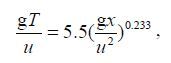 (4)
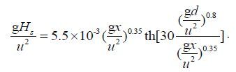
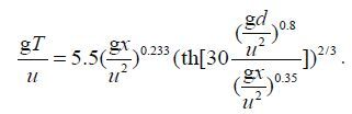
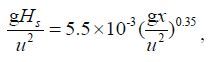
(4)where, H s, T, g, d denote significant wave height, period, gravitational acceleration and water depth respectively. Fetch lengths were prepared in advance in eight directions as a background data set. For both deep and shallow water, the following wave heightperiod relationship exists:
 (5)
(5)After wave height and period were computed, wave frequency and wave number were calculated by
 (6)
(6) (7)
(7)The forecasted H s, T, K were used in the oil spill forecast, which will be described in the oil spill model (Section 2.2).
Figure 1 shows a comparison between the parametrical wind wave model outputs and observations. It can be seen that the parametrical wind wave model can basically capture the variations of ocean waves. The root mean squared error is 1.0 m for significant wave height and 1.4 s for significant wave period. These accuracies can preliminarily meet the demands of an oil spill model to calculate the vertical eddy diffusivity and mixing of the oil spill into the water volume. The timesaving parametrical wind wave model takes less than one minute to predict 3 days, whereas in contrast, the numerical wave forecast model takes several hours. Faced with the demand for a quick response to an emergency oil spill, the parametrical wind wave model is acceptable and serviceable.

|
| Figure 1 Comparison between model outputs(red line)and observation(black line with asterisk) |
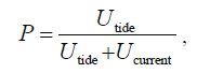
The sea surface current forecast model consists of a tidal current model, a circulation model and a wind drift model. This oil spill forecast system was developed to focus on oil slicks at the sea surface of Chinese offshore waters, where the tidal current model plays an essential role in coastal dynamic processes. Thus, for short term forecasting(several hours), the tidal current forecast model is key in oil spill drifting, however, for longer-term forecasting (several days), residual currents and wind drifting velocity are more important. Figure 2 shows the percentage of the tidal current that accounts for the sea surface current analyzed based on the operational tidal current forecast system(Fang et al., 2008)and an ocean general circulation model(Wang et al., 2006)by Eq.8.
 (8)
(8)

|
| Figure 2 The ratio of tidal current to sea surface current |
where U tide is the maximum possible tidal speed, U current is the annual mean speed of circulation. The tidal current accounted for over 80% of the sea surface currents in most parts of northern 30°N and the Beibu Gulf. On the coasts of Fujian Province, this percentage is usually between 60% and 80%, whereas it is around 50% in the coastal region of Guangdong Province.
To correspond with the emergency services, the quick forecast technique was selected to forecast sea surface currents based on residual currents and tidal current harmonic constants, using Eq.9a and 9b.
 (9a)
(9a) (9b)
(9b)where U(t)and V(t)denote the forecasted eastward and northward current. U 0 and V 0 are eastward and northward residual current, the subscript i represents the tidal constituents, U, ξ and V, η are the amplitude and phase lag for eastward and northward of tidal current, ω is the angular speed, v 0 is the initial phase of the equilibrium tide. f is the nodal fact, and u is the nodal adjustment angle of the initial phase.
For the residual current(U 0 and V 0), one source was derived from the forecast product of an operational ocean environmental forecast system(Wei et al.,2015), and the other source was derived from the climatological monthly mean surface current, which originated from an ocean general circulation model. At present, the second interface is used as the default option to fulfil the quick forecast demand. Figure 3 shows the surface residual current based on the variable grid global ocean model(Wang et al., 2006; Fang et al., 2009). It can be seen that the sea surface currents of offshore China are a typical, monsooncontrolled circulation. In winter, the sea surface currents are prevailingly southwest in the coastal region, except for in the Taiwan Strait. In the Bohai Sea, the sea surface currents exhibit weak circulation and the residual speeds are less than 0.1 m/s. At the west and north coast of the Yellow Sea, the sea surface currents also show weak circulation. For the rest region of the Yellow Sea, the sea surface currents are less than 0.2 m/s. In the west part of the East China Sea, the sea surface currents are fairly strong, with speeds greater than 0.2 m/s. In the northern South China Sea(except for the Beibu Gulf), the sea surface currents are stronger than in other coastal region. In the summer, the sea surface currents are basically weaker than in the winter, and are in the reverse direction. The sea surface currents in most of the coastal region are less than 0.1 m/s except for offshore of Zhejiang and Fujian Provinces. The sea surface currents are in transition conditions in the spring and autumn. As the sea surface currents of offshore China (especially for the Bohai Sea, Yellow Sea and East China Sea)are weak and dominated by monsoon, the residual currents, which are interpolated from climatological monthly mean current, can be used for the oil spill forecast system.

|
| Figure 3 Seasonal variations in sea surface currents(a)winter, (b)spring, (c)summer, (d)autumn |
The tidal currents forecast model was based on the numerical simulation results for China’s adjacent seas (Fang et al., 2008). The tidal ellipses for the principal tides of offshore China are shown in Fig. 4, with different scales for each tidal constituent. It can be seen that the semi-diurnal tidal current dominated the surface tidal currents of the East China Seas, except for in a small region near the Bohai Strait. On the contrary, the tidal current in the Beibu Gulf was controlled by the diurnal tidal current.

|
| Figure 4 Surface tidal current ellipses, (a)M 2, (b)S 2, (c)K 1, (d)O 1 |
To evaluate the tidal current constituents, over 350 stations of tidal current constituents(Fig. 5)were selected and compared with model results. To demonstrate the comparisons, the tidal current constituents were separated into a 1, a 2, a 3 and a 4 using Eq.10 for the eastern(U, ξ)and northern(V, η)tidal current constituents:
 (10a)
(10a) (10b)
(10b) (10c)
(10c) (10d)
(10d)

|
| Figure 5 Stations of tidal current constituents |
Figure 6 is the scattered diagram of the separated values(a 1, a 2, a 3 and a 4)for the principal semidiurnal tidal current M 2 and principal diurnal tidal current O 1 . Abscissa represents observed values and ordinate represents model results. It can be seen that most of the scattered points are near the diagonal line(the red solid line), indicating the reliable model results.

|
| Figure 6 Comparison between model results and observations, (a)M 2 and(b)O 1 |
To evaluate the validation of the current forecast model, four sea current observation stations(Fig. 7) were used for time series comparison of current speed and direction(Fig. 8). The default interface was selected for the residual current(U 0 and V 0 in Eq.9), which was derived from climatological monthly mean surface currents. Table 1 shows the mean absolute errors and root mean squared(RMS)errors of speed and direction for sea current forecast. The mean absolute error of current speed was 4.6 cm/s and the mean absolute error of current direction was 12.0°. The RMS of current speed was 5.7 cm/s and RMS of current direction was 16.9°. It can be suggested that the second interface of the residual current is suitable for most parts of offshore China. However, for the offshore region of the northern South China Sea, where circulation is vigorous and complicated, the first interface was more favorable.

|
| Figure 7 Stations used for sea current observations |

|
| Figure 8 Comparisons of the sea currents |

The oil spill model was based on the “particle method”, which represents the oil spill as a large number of particles. The drifting velocity, evaporation and emulsification processes control the evolution of each oil particle.
2.2.1 Horizontal and vertical movement of the oil spillThe drifting velocity of oil particle U p(t)and V p(t) can be denoted as:
 (11)
(11)where U(t)and V(t)are the background currents provided by the sea surface current forecast model
(Eq.9), U d(t)and V d(t)are wind drifting velocities, and U′(t)and V ′(t)are random turbulent velocities of the oil particles.
The horizontal movements of the oil particles within a sub-grid can be calculated through the following equations:
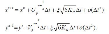 (12)
(12)We adopt central difference in time t to ensure the above difference equations to be of a second order accuracy. ξ, K H in the Eq.12 denotes the uniformly distributed random number in [-1, 1] and the horizontal eddy viscosity, respectively.
As the sea surface usually becomes smoother when covered by the spilled oil, the value of wave induced flow will be much smaller than that of the background current. Waves mainly affect the oil spill via the mixing effect and wave breaking, which induce some of the oil spill mixing into the water. The volume of the oil particle mixed into water is:
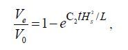 (13)
(13)where V 0, t, H s, L are the initial volumes of the oil spill, time, significant wave height and wave length (provided by parametrical wind wave model) respectively, and C 2 is a constant, -2.53×10 -3 / V 0 0.62 .
The oil spill mixed into water can be represented by oil drops, which are much smaller than the oil particle. The vertical displacement of oil drops can be calculated by Eq.14, where W b is the vertical velocity of an oil drop, W L is the floating velocity caused by the buoyancy, and K V is the vertical eddy viscosity.
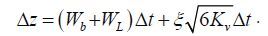 (14)
(14)The vertical eddy viscosity is derived from the Reynolds stresses, due to surface waves(Ichiye, 1967):
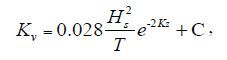 (15)
(15)where H s, T, Z, K are significant wave heights, wave periods, water depth and wave number, respectively, and C is a constant.
The float velocity was calculated on the basis of the diameter of each oil drop. Under the action of buoyancy, assuming the critical diameter of the oil drop is de, we have:
 (16)
(16)when di < de and Stokes law is applied, leading to:
 (17)
(17)when d i > d e
 (18)
(18)where g, d i, ν, ρ o, ρW are gravity accelerators, the diameter of oil drops, kinetic viscosity, the density of oil and the density of water, respectively.
Thus, the vertical coordinates of oil drops can be calculated through the following equation:
 (19)
(19)The evaporation and emulsification of the oil are related to the oil properties. The rate of evaporation can be written as follows(Stiver and Mackay, 1984):
 (20)
(20)where A′=6.3, B′=10.3, T is the temperature of spilled oil, T G is the curve gradient of the oil boiling point, T o is the initial boiling point of the oil, and θ′ is the coefficient of evaporation, which was defined by the following equation(Buchanan and Hurford, 1988):
 (21)
(21)where C is a constant, W is wind speed, t is time, A is the area of the oil slick, and V o is the initial volume of the oil spill.
The effect of emulsification is defined by the moisture content Y W, following Mackay et al.(1980):
 (22)
(22)where Y W is the moisture content in the emulsion, K A is taken as 4.5×10 -6, K B is taken as 1/ Y F W, in which Y F W is the final moisture content and is taken as 1.25.
Thus the volume of oil particles on the sea surface should be:
 (23)
(23)APPLICATION A graphical user interface(GUI)of the oil spill forecast system was designed using Visual C++. Figure 9 shows the main interface of the system.

|
| Figure 9 Main interface of the oil spill forecast system |
The main menu of the system includes six parts. The first menu is “File”. It presents the oil spill forecast service, which is the most fundamental function of the system. The second menu can set the display settings, such as zoom in, zoom out and selective amplification. The third menu controls the display information of the forecasted oil spill, such as the oil spill trajectory, the shape of the oil slick and the scatter of the oil particles. The fourth menu gives some information on decision support, including the handbook of emergency equipment and some emergency preplans. The fifth menu is the management of the database of the system. The oil spill forecast system embeds a database to manage the properties of oil(useful for forecasting the rate of evaporation), a reserve of emergency equipment and the distribution of the marine petroleum platforms. The sixth menu contains a user guide for this system.
Figure 10 shows a demonstration of the oil spill forecast system. The system can quickly forecast the trajectory of spilled oil and provide the shape of the oil slick, the residual quantity of spilled oil, and affected areas. Other serviceable information, such as positions of petroleum platforms, oil pipelines, and emergency equipment bases, can be displayed simultaneously.

|
| Figure 10 Demonstration of an oil spill forecast |
An oil spill emergency exercise was held at 125°00′35.82″E, 28°30′47.82″N, in the East China Sea, on 20th August, 2008. A tracer was released and tracked by the Hai Yang Shi You 689 ship(Fig. 11a). Prior to this emergency exercise, the trajectory of the oil spill was forecasted by our oil spill forecast system (the brown line in Fig. 11b). During the emergency exercise, we tracked the tracer and recorded the position hourly(the white line in Fig. 11b). Based on this oil spill emergency exercise, the average Lagrangian separation distance was 1.56 km. To evaluate the performance of the oil spill model, the skill score, as proposed in Liu and Weisberg(2011), was used. The skill score ss for the trajectory model is defined by Eq.24, where s is a non-dimensional index (defined as Eq.25), n is a positive number that defines the threshold of no skill, d i is the separation distance between the forecasted and observed track at time step i, and l oi is length of the observed trajectory. In this paper we chose n =1, and a skill score of 0.15 for this oil spill emergency exercise. According to the application on this oil spill emergency exercise, the developed oil spill forecast system exhibited a good performance and was able to satisfy an oil spill emergency response.
 (24)
(24) (25)
(25)

|
| Figure 11 Oil spill emergency exercise(a)and validation of the oil spill forecast system(b) |
A numerical model for an oil spill was described, which included an ocean environmental forecast model and an oil spill model. The timesaving ocean environmental forecast model comprised a parametrical wind wave forecast model and a sea surface current forecast model, and considered the demand for a quick response to the emergency event of oil spill. The oil spill model was based on the “particle method”. The evolution of each oil particle is controlled by drifting velocity, evaporation and emulsification processes. The GUI for an oil spill, based on these numerical models, is also described. Significant information, such as the properties of oil, emergency equipment reserves and distribution of marine petroleum platforms, were embedded into the system with a manageable database. The oil spill forecast system was successfully applied for an oil spill emergency exercise, and provides an operational service in the Research and Development Center for Offshore Oil Safety and Environmental Technology.
As described in Section 2.1, two interfaces were designed for the residual current(U 0 and V 0)in the sea surface current forecast model. The second interface, which was based on a climatological monthly mean surface current, was set to the default option. Although this default option shows some satisfactory results in the East China Seas(the Bohai Sea, Yellow Sea and East China Sea), the first interface, which was derived from the operational ocean environmental forecast system with multiple model ensemble(Liu et al., 2011c), is more favorable. Although the oil spill forecast system was validated by an oil spill emergency exercise, more extensive validations should be implemented using the skill scores, as proposed in Liu and Weisberg(2011).
As re-initialized locations of oil spills, duly obtained from oil spill monitoring systems, are critical components of the oil spill forecast system(Liu et al., 2011a), combined with an operational oil spill monitoring system was planned to implement in following development. We found that the oil spill model was suitable for forecasting the drifting and spreading of the spilled oil on the sea surface. However, we also found that when the spilled oil was attached to the coastline, the oil spill model was not very good at forecasting, because it is very difficult to determine how much oil will remain on the coastline, and how much oil will move back to the ocean. Therefore, we are still developing the oil spill numerical model, to improve its usability and accuracy.
| An W, Wang Y G, Wang X Y, Niu Z G, Zhao Y P, 2010. An oil spill forecast and emergency decision support system in China offshore. Marine Sciences, 34 (11) : 78 –83. |
| Buchanan I, Hurford N, 1988. Methods for predicting the physical changes in oil spilt at sea. Oil and Chemical Pollution, 4 (4) : 311 –328. Doi: 10.1016/S0269-8579(88)80004-2 |
| Cai Y, Mu L, Li H, Song J, Chi Y X, Guan C Y, Li C, 2013. A review of numerical modeling research on the marine oil spill. Marine Science Bulletin, 15 (2) : 71 –86. |
| Fang G H, Wang Y G, Wei Z X, Fang Y, Qiao F L, Hu X M, 2009. Interocean circulation and heat and freshwater budgets of the South China Sea based on a numerical model. Dyn. Atmos. Oceans, 47 (1-3) : 55 –72. Doi: 10.1016/j.dynatmoce.2008.09.003 |
| Fang G H, Wei Z X, Wang Y G, 2008. Development of tide and tidal current regional prediction in China. Advance in Earth Science, 23 (4) : 331 –336. |
| Gu E H, Yao Y M, 2013. Fractal simulation of oil spill trajectory in the northern port area of the Yueqing Bay. Marine Science Bulletin, 32 (4) : 460 –466. |
| Ichiye T, 1967. Upper ocean boundary-layer flow determined by dye diffusion. The Physics of Fluids, 10 (9) : S270 –S277. Doi: 10.1063/1.1762467 |
| Li D M, Liu J C, Wu D, Bai L, 2012. Mathematical model of marine oil spill in Bohai. Journal of Tianjin University, 45 (1) : 50 –57. |
| Li T, Xie Z Y, 2013. Study and application of oil spill trajectory model. Environmental Science and Management, 38 (7) : 56 –61. |
| Li Y, Zhu J, Wang H, Kuang X D, 2013. The error source analysis of oil spill transport modeling: a case study. Acta Oceanol. Sin., 32 (10) : 41 –47. Doi: 10.1007/s13131-013-0364-7 |
| Li Y, Zhu J, Wang H, Lin C Y, 2014. The assimilation technology application in the oil spill emergency forecasting system of the Bohai Sea. Acta Oceanol. Sin., 36 (3) : 113 –120. |
| Liu Y G, MacFadyen A, Ji Z G, Weisberg R H, 2011a. Trajectory forecast as a rapid response to the Deepwater Horizon oil spill. In: Liu Y G, Weisberg R H, Hu C M, Zheng L Y eds. Monitoring and Modeling the Deepwater Horizon Oil Spill: A Record-Breaking Enterprise. American Geophysical Union, 195 : 153 –165. Doi: 10.1029/GM195 |
| Liu Y G, MacFadyen A, Ji Z G, Weisberg R H. 2011b. Monitoring and Modeling the Deepwater Horizon Oil Spill: A Record-Breaking Enterprise. AGU/Geopress, Washington D.C., http://dx.doi.org/10.1029/GM195. |
| Liu Y G, Weisberg R H, Hu C M, Zheng L Y, 2011c. Tracking the deepwater horizon oil spill: a modeling perspective. Eos Trans., AGU, 92 (6) : 45 –46. Doi: 10.1029/2011EO060001 |
| Liu Y G, Weisberg R H, 2011. Evaluation of trajectory modeling in different dynamic regions using normalized cumulative Lagrangian separation. J. Geophys. Res, 116 (C9) . |
| Mackay D, Paterson S, Trudel K. 1980. A Mathematical Model of Oil Spill Behavior. Environmental Protection Services. Fisheries and Environment, Canada. |
| Mu L, Wu S Q, Song J, Li H, Liu S H, Li Y, Gao J, 2011a. Numerical model research on Emergency Warning and Predicting system of ocean oil spill: I. Research on predicting of ocean dynamical factors. Marine Science Bulletin, 30 (5) : 502 –508. |
| Mu L, Wu S Q, Song J, Li H, Liu S H, Li Y, Gao J, 2011b. Numerical model research on Emergency Warning and Predicting system of ocean oil spill in Bohai Sea: II. The visualization and the research on application. Marine Science Bulletin, 30 (6) : 713 –717. |
| Röhrs J, Chistensen K H, Hole L R, Broström G, Drivdal M, Sundby S, 2012. Observation-based evaluation of surface wave effects on currents and trajectory forecasts. Ocean Dynamics, 62 (10-12) : 1519 –1533. Doi: 10.1007/s10236-012-0576-y |
| Stiver W, Mackay D, 1984. Evaporation rate of spills of hydrocarbons and petroleum mixtures. Environmental Science & Technology, 18 (11) : 834 –840. |
| Wang Y G, Fang G H, Wei Z X, Qiao F L, Chen H Y, 2006. Interannual variation of the South China Sea circulation and its relation to El Niño, as seen from a variable grid global ocean model. J. Geophys. Res., 111 (C11) : C11S14 . |
| Wei Z X, Xu T F, Wang Y G, Li H P, Yang X L, Feng W Z, Zhang Z Y, 2015. Introduction to the fine-resolution windwave-current coupled forecasting and information service system for the South China Sea and its adjacent seas areas. Journal of Ocean Technology, 34 (3) : 86 –90. |
| Wen S C, Zhang D C, Chen B H, Gao P F, 1989. A hybrid model for numerical wave forecasting and its implementation: Part I, the wind wave model. Acta Oceanol. Sin., 8 (1) : 1 –14. |