 2016, Vol. 34
Institute of Oceanology, Chinese Academy of Sciences
Article Information
- KONG Fanzhou(孔凡洲), XU Zijun(徐子钧), YU Rencheng(于仁成), YUAN Yongquan(袁涌铨), ZHOU Mingjiang(周名江)
- Distribution patterns of phytoplankton in the Changjiang River estuary and adjacent waters in spring 2009
- Chinese Journal of Oceanology and Limnology, 34(5): 902-914
- http://dx.doi.org/10.1007/s00343-016-4202-6
Article History
- Received Aug. 1, 2014
- accepted in principle Oct. 2, 2014
- accepted for publication Jul. 14, 2015


2 Laboratory of Marine Ecology and Environmental Science, Qingdao National Laboratory for Marine Science and Technology, Qingdao 266071, China;
3 North China Sea Monitoring Centre, Qingdao 266033, China
The Changjiang (Yangtze) River is the longest river in China, with a drainage area of 1.8 million km2. Large quantities of nutrients are transported into the sea through the Changjiang River, and this area forms an important basis for the Zhoushan fishing ground. However, the quantity of nutrients discharged into the estuary and its adjacent waters has significantly increased with the rapid development of industry and agriculture in the drainage basin of the Changjiang River, and resulted in the serious problems with eutrophication and red tides (Wang et al., 2002; Wang, 2007; Pei et al., 2009). A red tide is the abnormal phenomenon of seawater discoloration caused by excessive growth or accumulation of microscopic plankton. Some red tides, generally termed as harmful algal blooms, bring deleterious impacts on marine organisms and ecosystems, and subsequently human health (GEOHAB, 2001).
The Changjiang River estuary (CRE) and adjacent waters are among the most notable regions for red tides in the coastal waters of China. Large scale red tides of Prorocentrum donghaiense have been recorded every spring in the coastal waters adjacent to the CRE since 2000, and the maximum affected sea area is, at times, over 10 000 km2 (Zhou and Yu, 2007). Red tides were mainly found in the sea area with abrupt changes in bottom topography at depths of 30–50 m (Zhou et al., 2003; Tang et al., 2006). In the spring, red tides of both diatoms and dinoflagellates were found in this region, and there was an apparent succession of red tide causative species from diatoms to dinoflagellates from March to May (Zhou et al., 2008). With increasing water temperature and light intensity, diatoms take advantage of the nutrients accumulated over the winter and grow rapidly to form the first red tides. Once nutrients, particularly phosphate, are consumed to a low level, and thus the growth of diatoms is limited, the diatom red tide will reduce in size. Subsequently, with the continuous increase in water temperature and the occurrence of stratification, red tides of dinoflagellates appear (Zhou and Zhu, 2006). There is a high frequency of red tides and other abnormal ecological events, such as jellyfish blooms and hypoxia, occurring in the sea area adjacent to the CRE. This has caused this region to become a hot spot in marine ecological studies in China since the beginning of the new millennium (Shen and Hong, 1994; Huang et al., 2000; Wang and Huang, 2003).
Many investigations have been performed in the CRE and its adjacent waters during the last few decades because of the ecological significance of this region. In phytoplankton ecological studies conducted prior to the appearance of massive dinoflagellate red tides in this region around the year 2000, most samples were collected with a phytoplankton net (nominal pore size at 67 μm) (Wu et al., 2000). Those netconcentrated samples, however, are not suitable for studies of dinoflagellate red tides, because the bloomforming species like P. donghaiense, Karenia mikimotoi, Gyrodinium spirale, Scrippsiella trochoidea and Alexandrium spp. in the CRE and adjacent waters are generally less than 70 μm in cell size. Additionally, there is no information on the vertical distribution of red tides using net-concentrated samples. Therefore, the collection of discrete water samples are gradually accepted in phytoplankton investigations (Gao and Song, 2005; Chen et al., 2006; Luan et al., 2006; He et al., 2009; Zhao et al., 2010; Sun and Tian, 2011) and red tide studies in the CRE and adjacent waters.
To understand the phytoplankton distribution patterns, statistical methods like cluster analysis are often adopted. Cluster analysis has been widely used in marine ecological studies of planktonic and benthic communities. This method was used to analyze netconcentrated phytoplankton samples in the CRE and adjacent waters, and the phytoplankton assemblage was classified into “freshwater community”, “estuary community” and “offshore community” (Guo and Yang, 1992; Wu et al., 2000; Wang, 2002). However, the application of such methods to analyze discrete water samples of phytoplankton in the sea area adjacent to the CRE is still quite limited (Zhao et al., 2010).
A comprehensive survey was carried out from 7 to 18 May in 2009 in the CRE and adjacent waters (30°30′–32°00′N, 122°00′–123°20′E). Discrete water samples were collected during the cruise, and phytoplankton taxa and abundance were determined by microscope. Cluster analysis and non-metric multidimensional scaling (NMDS) were conducted on a data matrix that included taxa composition and cell abundance of the phytoplankton samples. The purpose of this study was to reveal the distribution patterns of phytoplankton, and their relationship with environmental factors in the CRE and adjacent waters.
2 MATERIAL AND METHOD 2.1 Study areaThe study area, located in the CRE and adjacent coastal waters (30°30′–32°00′N, 122°00′–123°20′E), is illustrated in Fig. 1. The average depth of the study area was about 30 m, and the sea bottom topography was characterized by a sharp gradient between longitudes 122o30′E and 123o00′E (water depth 20–60 m). This area is significantly affected by freshwater discharge from the Changjiang River as well as seasonal upwelling, resulting in a rich biodiversity of phytoplankton. Large quantities of nutrients transported into this area by the Changjiang River make this a highly productive region. The overenrichment of nutrients, however, has caused this region the most notable red tide zone in the coastal waters of China after the year 2000.

|
| Figure 1 Study area and sampling sites Depth contours of the study area are marked in grey lines. |
Phytoplankton samples (n=72) were collected from the surface and at different depths (10 m, 30 m, and in the bottom layer about 2 m above seafloor), using water samplers installed on an ALEC CTD (JFE Advantech Co. Ltd., Nishinomiya, Japan) at 24 sampling sites. The water samples (0.5 L) were fixed with 6–8 mL Lugol’s solution and stored at room temperature. Concentrating phytoplankton in water samples was achieved using Utermöl’s methods (Utermöhl, 1958). Briefly, 25 mL well-mixed water sample was placed into a sedimentation chamber and settled for 24 h (Lund et al., 1958). The microalgae were then identified and counted under an inverted microscope.
To accurately depict the complex hydrological conditions, hydrological variables, such as seawater temperature, salinity and turbidity (NTU), were obtained from the 34 sampling sites (Fig. 1) using the ALEC CTD. Measurements were made at the same depths as the collection of water samples and at additional depths at 5 m and 20 m.
2.3 Data analysis 2.3.1 Biodiversity indicesThe Margalef index (dMa) (Margalef, 1958), Shannon index (H) (Shannon, 1948), Pielou evenness index (J) (Pielou, 1966) and dominance index (Yi) (McNaughton, 1967) were used to represent the biodiversity of the phytoplankton community. The Margalef index (dMa) reflects species richness using the number of phytoplankton species and the abundance of phytoplankton. The Shannon index (H) is used to measure the species biodiversity of a sample. The Pielou evenness index (J) indicates the species distribution evenness in the community. The dominance index (Yi) helped to determine the dominant species, and excluded interference of rare species for data analysis. Indices dMa, H and J were calculated with Biodixcel.xlsx (Kong et al., 2012), with the following formulae:
 (1)
(1) (2)
(2) (3)
(3) (4)
(4)where S is the total number of phytoplankton species, N is the abundance of phytoplankton, Pi is the proportion of individuals belonging to the ith species in the dataset of interest, ni is the abundance of the ith species, and fi is the frequency of the ith species occurring in the samples.
2.3.2 Cluster analysis and non-metric multidimensional scalingData analysis was conducted on a data matrix that included both taxa composition and cell abundance in the 72 phytoplankton samples collected from 24 sites. Rare species with a frequency below 10% were not taken into consideration. A standardized triangle similarity matrix was constructed through the BrayCurtis similarity measure, and fourth root transformation analysis was adopted to balance rare and common species. Based on Bray-Curtis similarities, hierarchical clustering with groupaverage linking was constructed. However, cluster analysis itself, which shows the similarities of the samples in the same group in one-dimensional quality level, is not enough to reflect the characteristics of the whole community. Therefore, cluster analysis was used in conjunction with NMDS and analysis of similarity (ANOSIM) methods. The samples were ordinated by NMDS in a two-dimensional map. The stress coefficient (s) of the ordination, in the case of NMDS, indicates excellent representation (s < 0.05), adequate ordination (s < 0.2) or arbitrary ordination (s > 0.3) (Clarke and Warwick, 2001). ANOSIM analysis was used to test the significance of difference among the clusters, and SIMPER analysis was used to compare average abundance and examine the contribution of each species to similarities within a given group, or dissimilarities between groups (Clarke and Warwick, 2001). The above analyses were performed with PRIMER 6.0 software (Clarke and Gorley, 2006). To prepare the contour maps for cell abundance and different hydrological variables, Surfer 11 was used with the Kriging gridding method.
3 RESULT 3.1 Hydrological conditions at the study areaThe water temperature, salinity and turbidity in the study area are illustrated in Fig. 2. Water temperature at the surface ranged from 18.4–21.1°C, while for most of the sampling sites, water temperature was between 19.0–19.5°C. Water temperature was generally higher in the southern part of the study area than in the northern part (Fig. 2a). However, there was an obvious low-temperature area around sampling site 32 in the southern part of the study area.

|
| Figure 2 Horizontal distribution of temperature (a), salinity (b) and turbidity (c) at the surface in the study area |
Salinity in the study area ranged from 7.9–30.06. Salinity increased gradually from the estuary to the offshore area, forming a bifurcation near sampling site 15, and an area with dense isohalines along the longitude 122 °30′E (Fig. 2b).
Turbidity in the study area ranged from 0–1820 NTU. The diluted water at the southern branch from the bifurcation point had much higher turbidity and affected a large sea area. The high turbidity area was distributed mainly at the entrance of the CRE (Fig. 2c), the entrance of Hangzhou Bay and the area around the Shengsi Islands. Turbidity in the sea area east of latitude 122.4°E decreased rapidly to below 10 NTU.
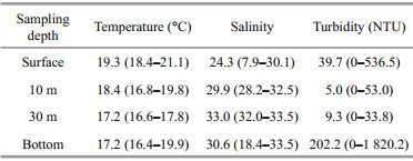
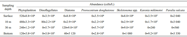
Temperature, salinity and turbidity at different sampling depths are shown in Table 1. Obvious halocline and thermocline layers could be observed. The temperature was about 2°C higher at the surface than at the bottom, while salinity at the surface was much lower than the bottom, reflecting stratification under the influence of the Changjiang River diluted water.
 |
In the 72 phytoplankton samples, 94 taxa were identified, including 52 taxa of diatoms, 40 taxa of dinoflagellates, and two species of chrysophytes. Diatoms and dinoflagellates dominated the phytoplankton assemblage in the CRE and adjacent coastal waters.
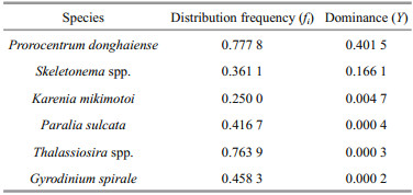
Dominant microalgae, defined by a dominance index Yi higher than 0.000 2, are listed in Table 2. The dominant phytoplankton taxa were, in descending order, P. donghaiense, Skeletonema spp., K. mikimotoi, Paralia sulcata, Thalassiosira spp. and Gyrodinium spirale.
Average phytoplankton abundance in the study area was 46.0 (0.012–883.8)×104 cells/L. The abundance of diatoms and dinoflagellates was 21.26 (0–883)×104 cells/L and 24.7 (0–351)×104 cells/L, respectively, accounting for 46%(0–100%) and 53.7% (0–92%) of the total abundance of phytoplankton. In the surface seawater, phytoplankton abundance was 85.8 (0.05–883)×104 cells/L, while the abundances of diatoms and dinoflagellates were 47.3 (0–883)×104 cells/L and 38.5 (0–350)×104 cells/L, respectively. With respect to the dominant taxa, the abundances of P. donghaiense, Skeletonema spp. and K. mikimotoi were 36.8 (0–350), 47.1 (0–883) and 1.5 (0–35)×104 cells/L, respectively.
The distributions of major phytoplankton groups and dominant microalgal taxa at the surface are shown in Fig. 3. The horizontal distribution patterns of diatoms and dinoflagellates coincide well with their dominant species, Skeletonema spp. and P. donghaiense.

|
| Figure 3 Distribution of major phytoplankton groups and dominant microalgal species at the surface in the study area (abundance, ×104 cells/L) a. total phytoplankton; b. diatoms; c. Skeletonema spp.; d. dinoflagellates; e. Prorocentrum donghaiense; and f. Karenia mikimotoi. Bold lines in (c), (e) and (f) indicate the distribution of red tides of Skeletonema spp., Prorocentrum donghaiense and Karenia mikimotoi. |
The vertical distribution of major phytoplankton groups and dominant taxa are listed in Table 3. The abundance of both dinoflagellates and diatoms decreased with water depth, and the minimum value of diatoms appeared at 30 m depth.
According to the cluster analysis (Fig. 4), phytoplankton samples collected from the study area could be divided into three major clusters (Group Ⅰ– Ⅲ) at a similarity level of 30%, except for 1 sample collected at a depth of 10 m from sampling site 42 (sample T42 on the left of the dendrogram). Group Ⅰ included 16 samples evenly arranged in the dendrogram with a low similarity level. Group Ⅱ included five samples with a similarity level of around 70%. Group Ⅲ had 50 samples, which could be further divided into two subgroups (Ⅲ-S1, Ⅲ-S2) at a similarity level of 40%.

|
| Figure 4 Clustering dendrogram of the phytoplankton community in the study area Samples were named after the sampling site codes and the sampling depth, where “S” for surface, “T” for 10 m depth, “Th” for 30 m depth and “B” for bottom. |
The non-metric multidimensional scaling map is shown in Fig. 5. Except for sample T42, which could be distinguished from other samples at a similarity of 20%, the other samples were classified into three groups at a similarity level around 30%. Each group took up a fixed position, although there was an overlap between Groups Ⅰ and Ⅲ. The two groups might be better distinguished in scaling analysis with more dimensions, but the 2-dimension scaling map was enough to demonstrate the similarity in each group of phytoplankton samples. The pressure coefficient (s) was 0.19, and therefore, the classification could reflect differences among the phytoplankton samples collected from the study area.

|
| Figure 5 NMDS ordination of the phytoplankton communities in the study area |
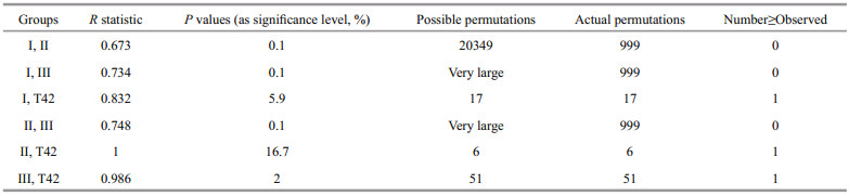
ANOSIM found significant differences among the groups (the value of global R was 0.749, P < 0.1%). Excluding sample T42, there were significant differences between any two selected groups (P < 0.1%) (Table 4), and therefore, the classification was credible.
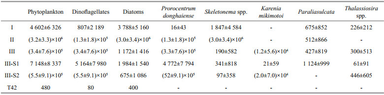
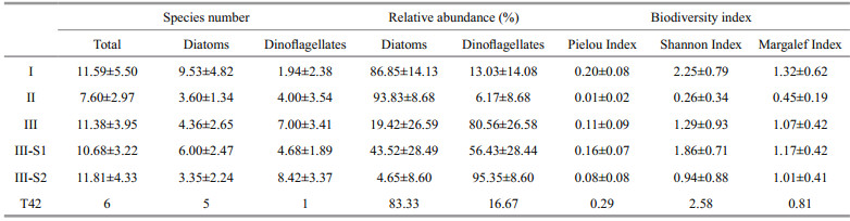
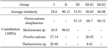
The dominant species, abundance, relative contribution of diatoms and dinoflagellates, and biodiversity indices for each group of phytoplankton samples are shown in Tables 5 and 6.
 |
 |
Among the three groups, Group Ⅰ possessed the highest biodiversity, but the lowest abundance of phytoplankton. Phytoplankton samples in Group Ⅰ were dominated by diatoms, and the dominant taxa were Skeletonema spp., P. sulcata, Chaetoceros spp., Thalassiosira spp., Nitzschia spp. and Coscinodiscus spp., with abundances of 1 847, 675, 282, 226, 118 and 104 cells/L, respectively. Skeletonema spp. accounted for around 50% of the total diatom cells.
Samples from Group Ⅱ had the lowest biodiversity, and Skeletonema spp. dominated all phytoplankton samples. On average, the abundance of Skeletonema spp. was 3.2×10⁶ cells/L, which accounted for 94% of the total phytoplankton cells. The abundance of dinoflagellate P. donghaiense was 1.2×10⁵ cells/L, accounted for only 6% of the total phytoplankton cells. The abundance of other microalgal species was much lower compared with Skeletonema spp. and P. donghaiense. Those species with abundances higher than 100 cells/L were P. sulcata, Thalassiosira spp., Melosira sp. and Prorocentrum minimum.
The samples from Group Ⅲ were characterized by a high proportion of dinoflagellates. This group was further divided into two subgroups. The phytoplankton abundances in the samples from subgroup Ⅲ-S1 were relatively low (7 145 cells/L), and the dominant species were P. donghaiense and P. sulcata. The presence of the benthic diatom Paralia sulcata was the major characteristic of subgroup Ⅲ-S1. Other taxa, including Skeletonema spp., Thalassiosira spp. and S. trochoidea, were also present in Ⅲ-S1, with abundances of 341, 238 and 92 cells/L, respectively.
Samples in subgroup Ⅲ-S2 were characterized by a high abundance of dinoflagellates. On average, phytoplankton abundance was 55.0×10⁴ cells/L, in which dinoflagellates accounted for more than 95%. Prorocentrum donghaiense was the dominant species, with an abundance of 52.7×10⁴ cells/L. Karenia mikimotoi took second place, with an abundance of 2.0×10⁴cells/L. Other species with abundances higher than 100 cells/L were G. spirale (446 cells/L), P. minimum (226 cells/L), S. trochoidea (188 cells/L), G. instriatum (134 cells/L), and Protoperidinium spp. (105 cells/L). The abundance of diatoms in Ⅲ-S2 was much lower, and Thalassiosira spp. was the dominant diatom species. Skeletonema spp. was only found in a few samples from subgroup Ⅲ-S2 in the northern part of the study area.
Sample T42 was quite different from the rest of the samples collected from the CRE and adjacent waters. Only four taxa (Prorocentru m sp., Coscinodiscus jonesianus, Nitzschia sp. and Diploneis sp.) were identified in this sample, and the abundance of phytoplankton was extremely low (below 80 cell/L for every species).
Biodiversity indices, namely the Pielou evenness index, Shannon index and Margalef index, were also similar within groups, but exhibited clear differences among groups (Table 6).
SIMPER analysis of the species-by-sample matrix was used to determine the species representing each group. Table 7 displays the average similarity of the four groups and the typical species contributing to the average within-group similarity. In Groups Ⅰ and Ⅱ, the average similarities were 28.6% and 90.1%, respectively. In Group Ⅲ, the average similarities were 50.7% and 66.1% for the two subgroups Ⅲ-S1 and Ⅲ-S2, respectively. Skeletonema sp., P. donghaiense, Paralia sulcata and Thalassiosira sp. were the most important species impacting similarities within each group.
 |
Horizontal and vertical distribution patterns of the three groups of phytoplankton community are shown in Figs. 6 and 7. Groups Ⅰ and Ⅱ were mainly distributed in the area west of 122°50′E. Group Ⅰ was centered around the river mouth and the Shengsi islands, while Group Ⅱ was situated around Group Ⅰ. Group Ⅲ was distributed further offshore compared with Groups Ⅰ and Ⅱ. Subgroup Ⅲ-S1 was mainly found at the surface in the sea area north to the Shengsi islands and at the bottom east of 122°50′E. Subgroup Ⅲ-S2 was mainly distributed at the surface, east of 122°50′E, but was also found west of 122°50′E in the northern part of the study area.

|
| Figure 6 Horizontal distribution of phytoplankton groups in surface waters |

|
| Figure 7 Vertical distribution of phytoplankton groups in different sections of the study area |
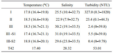
Environmental variables relating to the three phytoplankton groups are shown in Table 8. There were no apparent differences in seawater temperature among the groups, while salinity was significantly different among the groups. The salinities of Group Ⅰ and Ⅱ were 25.5 and 22.9, respectively, much lower than in Group Ⅲ. The turbidity associated with the different groups also exhibited clear differences, with a gradual decrease from Group Ⅰ to Group Ⅲ. Highest turbidity was observed in Group Ⅰ, with an average value of 327 NTU. The turbidity ranges associated with Group Ⅱ (0.1–44.3) and Group Ⅲ (0–39.8) were similar, but the average turbidity of Group Ⅱ (23.4) was markedly higher than Group Ⅲ.
 |
In this study, discrete phytoplankton samples were collected from the sea area adjacent to the CRE during the outbreak stage of red tides in May 2009. Altogether, 94 taxa of microalgae were identified, including the most important red tide causative species in this region: Skele tonema spp., P. donghaiense and K. mikimotoi. Zou (2004) suggested a criterion for defining red tides of S keletonema costatum (cell abundance higher than 5×10⁷ cells/L). For other microalgal species, the criteria have been suggested as 106 cells/L or 3×10⁵ cells/L for microalgae with cell sizes of 10–29 μm or 30–99 μm, respectively (Adachi, 1973). According to these criteria, four patches of red tides were found in the study area, formed by Skeletonema spp., P. donghaiense and K. mikimotoi. The Skeletonema spp. red tide occurred in the central part of the study area near sampling site 18. There were two red tide patches formed by P. donghaiense; one appeared in the sea area near sampling sites 2 and 3 in the northern part of the study area, and the other near sampling site 34 in the southern part of the study area. Another small red tide patch, formed by K. mikimotoi, was found near sampling site 19. Although K. mikimotoi had a relatively low cell density (maximum cell density at 3.5×10⁵ cells/L), it was the second dominant species of dinoflagellates in the phytoplankton community and an important fish-killing species. Therefore, the red tide formed by K. mikimotoi should not be neglected.
These red tides could be well represented by the groups/subgroups deduced from the cluster analysis of the phytoplankton samples. Based on the data matrix of taxa composition and abundance established in this study, the phytoplankton assemblage in the sea area adjacent to the CRE were classified into three groups at a similarity level of 30%, and Group Ⅲ could be further divided into two subgroups (Ⅲ-S1, Ⅲ-S2) at a similarity level of 40%. Group Ⅱ represented Skeletonema spp. red tide, and Subgroup Ⅲ-S2 represented dinoflagellate red tides of P. donghaiense and K. mikimotoi. Based on the distribution of different red tides, it can be seen that there was a gradual change in red tide causative species from the estuary to the offshore sea area, from diatoms to armored dinoflagellates and then unarmored dinoflagellates.
The CRE and its adjacent waters have a complex physical and chemical environment, affected by the Changjiang River diluted water, alongshore currents, and upwelling. Cluster analysis allowed us to relate the distribution of phytoplankton and red tides (as represented by different groups/subgroups) to environmental factors and processes, including salinity, turbidity, and upwelling.
4.1 Effects of temperature, salinity and turbidityBased on the environmental data, water temperature in the study area (16.4–21.1°C) did not affect the distribution of phytoplankton and red tides. The maximum difference in temperature among the three phytoplankton groups was only 0.7°C. According to previous studies, the optimal temperature for the growth of P. donghaiense is 22–28°C (Deng et al., 2009), but the growth of P. donghaiense would not be significantly limited when water temperature was higher than 15°C (Wang et al., 2006). Similarly, the optimal temperature for the growth of S. costatum is 22°C (Xu et al., 2010), and its growth rate at 16°C is similar to the maximum growth rate at 22°C (Chen et al., 2005). Therefore, water temperature in the study area is not a limiting factor for the growth of these red-tide causative species, and will not affect the distribution of red tides.
Salinity, however, was an important factor affecting the distribution of phytoplankton and red tides in the CRE and adjacent waters. Phytoplankton communities in the central and western parts of the study area were characterized by estuarine diatoms dominated by Skeletonema spp. Previous studies suggested that the diatom S. costatum can adapt to a wide range of salinities, and the optimal salinity range was 18–25.7 (Chen et al., 2005). In this study, Skeletonema spp. could be observed in Groups Ⅰ, Ⅱ and Subgroup Ⅲ-S1, with a wide salinity range. However, the optimal salinity range for the growth of P. donghaiense (25–31) was much narrower and higher than for the diatom S. costatum (Chen et al., 2005). Therefore, subgroup Ⅲ-S2, which was characterized by the P. donghaiense red tide was found further offshore and had a higher salinity value of 29.6.
The impacts of salinity on the distribution of phytoplankton and red tides may reflect the potential role of nutrients. Unfortunately, nutrient data were not available in this study. In previous studies in this region, however, it was found that nutrient concentration has a negative linear correlation with salinity (for example, Huang et al., 1986). Therefore, a decreasing trend of nutrient concentrations from the estuary to the offshore area can be expected. This trend is likely to affect the distribution of red tides, since the diatom Skeletonema spp. and dinoflagellate P. donghaiense have different nutrient utilization features. Skeletonema costatum can absorb nutrients rapidly (Wang et al., 2006), and the consensus is that diatoms grow much faster than dinoflagellates when there are enough nutrients available (Furnas, 1990). Therefore, red tides of Skeletonema spp. are often found in sea areas just outside the estuary, as observed in the current study. In the sea area further offshore, where nutrient concentration could limit the growth of diatoms, dinoflagellate P. donghaiense would have a greater opportunity to form red tides. This could account for the horizontal distribution patterns in red tides in the sea area adjacent to the CRE.
Turbidity was also a major limiting factor for the growth of phytoplankton in the estuary. In the CRE and adjacent waters, there was a negative relationship between turbidity and salinity. This is not unexpected, since both parameters are influenced by the Changjiang River runoff. The Changjiang River brings huge amounts of sand and silt into the East China Sea. The suspended materials will decrease the amount of photosynthetically active radiation entering the water. In the area near the estuary west of 122°E, the growth of phytoplankton is expected to be limited by light due to the high concentration of suspended substances (Shen, 1993). The horizontal gradient of suspended materials and a sediment front have been documented in the CRE and adjacent waters (Hu and Hu, 1995), influenced by the Changjiang plume and tide. Skeletonema spp. was the dominant species in both Groups Ⅰ and Ⅱ, but the average turbidity of Group Ⅱ was only 24.3 NTU, much lower than that of Group Ⅰ (327 NTU). The sharp decrease in turbidity seemed to be a major factor for the outbreak of the diatom red tide caused by Skeletonema spp. Prorocentrum donghaiense is adaptable to a wide range of illuminations (2–223 μmol/(m2·s)) (Xu et al., 2010), and thus light itself is unlikely to explain the varying distribution of red tides caused by Skeletonema spp. and P. donghaiense.
4.2 Effects of physical oceanographic processesPlume fronts, stratification and upwelling are important physical oceanographic phenomena and processes in the CRE and adjacent waters. A salinity value of 25 was often regarded as a convenient marker for the plume front, which can affect the biological, chemical and hydrological features of the estuary. The plume front zone, which has relatively low suspended matters and moderate nutrients for marine phytoplankton, has higher productivity (Hu and Hu, 1995). In this study, the 25-isohaline runs southwards from sites 2 to 32, fitting in well with the distribution of the diatom red tide (Group Ⅱ) and dinoflagellate red tide (Subgroup Ⅲ-S2).
Stratification and upwelling also appeared to play important roles in the distribution of phytoplankton communities. According to the vertical distribution of salinity (Fig. 8), seawater from the open ocean with high salinity formed a wedge from the seabed towards the estuary. Affected by the bottom topography at sampling sites 23–27 and 30–34, upwelling formed from May to August in an area centered at 31°30′N and 122°40′E (Zhao, 1993). Strong upwelling at sampling site 32 resulted in low-temperature and high-salinity seawater at the surface, and the presence of abundant benthic diatom P. sulcata. During the investigation, P. donghaiense was not the dominant species at sampling site 32, probably due to the mixing effects caused by upwelling and relatively high concentration of nutrients (Bu et al., 2005). In the sea area nearby, where the effects of upwelling declined and stratification developed, the relatively stable condition allowed P. donghaiense to form a red tide (Group Ⅲ-S2).

|
| Figure 8 Vertical profiles of salinity in sections along sampling sites 23–27 (a) and 30–34 (b) |
Considering the classification of phytoplankton assemblages and the effects of different environmental factors, it was suggested that phytoplankton Group Ⅰ is closely associated with turbidity, Group Ⅱ with turbidity, nutrients and plume front, subgroup Ⅲ-S1 with upwelling and stratification, and subgroup Ⅲ-S2 with salinity, nutrients and stratification.
5 CONCLUSION(1) During an investigation in the sea area adjacent to the CRE in May 2009, water samples were collected and phytoplankton taxa composition and abundance were determined. Red tides of diatoms Skeletonema spp. and dinoflagellates P. donghaiense and K. mikimotoi were observed. The red tide of Skeletonema spp. appeared in the front zone of the Changjiang River plume, associated with low salinity and high nutrient availability. The red tide of P. donghaiense was distributed further offshore, outside the plume front zone, in the sea area with high salinity and low turbidity where stratification was well developed. The red tide of K. mikimotoi was observed in the sea area associated with high salinity and relatively low nutrient availability. The causative species of red tides exhibited a gradual change from the estuary to the offshore sea area, from diatoms to armored dinoflagellates and then unarmored dinoflagellates;
(2) A data matrix, including taxa composition and cell abundance of the phytoplankton samples, was established and used for non-metric multidimensional scaling, cluster analysis, and analysis of similarities (ANOSIM). Analyses categorized the samples into three groups (Group Ⅰ, Ⅱ, Ⅲ) at the 30% similarity level. Group Ⅲ could be further divided into two subgroups (Ⅲ-S1, Ⅲ-S2). Group Ⅱ and subgroup Ⅲ-S2 could represent the red tides of diatoms Skeletonema spp. and dinoflagellates P. donghaiense and K. mikimotoi;
(3) Salinity, turbidity, plume front, upwelling, stratification and (probably) nutrients were important factors affecting the distribution of phytoplankton and red tides in the sea area adjacent to the CRE. Group Ⅰ was closely associated with turbidity, Group Ⅱ with turbidity, nutrients and plume front, subgroup Ⅲ-S1 with upwelling and stratification, and subgroup Ⅲ-S2 with salinity, nutrients and stratification.
6 ACKNOWLEDGEMENTThe authors thank Dr. LI Yang of South China Normal University for his help in diatom identification and Dr. LIU Xiaoshou of Ocean University of China for his assistance with PRIMER analysis.
| Adachi R, 1973. Organisms of red tide and actual situation of red tide. Fisheries Engineering, 9 (1) : 31 –36. |
| Bu X W, Xu W Y, Zhu D D, Chen G X, 2005. Discussion about mechanism of harmful algal blooms breakout. Acta Oceanol. Sin., 24 (1) : 101 –106. |
| Chen B Z, Wang Z L, Zhu M Y, Li R X, 2005. Effects of temperature and salinity on growth of Prorocentrum dentatum and comparisons between growths of Prorocentrum dentatum and Skeletonema costatum. Advances in Marine Science, 23 (1) : 60 –64. |
| Chen H L, Lv S H, Zhang C S, Zhou D D, 2006. A survey on the red tide of Prorocentrum donghaiense in East China Sea, 2004. Ecologic Science, 25 (3) : 226 –230. |
| Clarke K R, Gorley R N. 2006. PRIMER v6:User Manual/Tutorial. PRIMER-E, Plymouth. 192p. |
| Clarke K R, Warwick R M. 2001. Change in Marine Communities:An Approach to Statistical Analysis and Interpretation. 2nd edn. PRIMER-E, Plymouth. 172p. |
| Deng G, Geng Y H, Hu H J, Qi Y Z, Lv S H, Li Z K, Li Y G, 2009. Effects of environmental factors on photosynthesis of a high biomass bloom forming species Prorocentrum donghaiense. Marine Sciences, 33 (12) : 34 –39. |
| Furnas M J, 1990. In situ growth rates of marine phytoplankton:approaches to measurement, community and species growth rates. J. Plankton Res., 12 (6) : 1171 –1151. |
| Gao X L, Song J M, 2005. Phytoplankton distributions and their relationship with the environment in the Changjiang Estuary, China. M ar. P ollut. B ull., 50 (3) : 327 –335. |
| GEOHAB. 2001. Global ecology and oceanography of harmful algal blooms, science plan. I n:Glibert P, Pitcher G eds.SCOR and IOC. Baltimore and Paris. 87p. |
| Guo Y J, Yang Z Y, 1992. Quantitative variation and ecological analysis of phytoplankton in the estuarine area of the Changjiang River. Studia Marina Sinica, 33 : 168 –189. |
| He Q, Sun J, Luan Q S, Yu Z M, 2009. Phytoplankton in Changjiang Estuary and adjacent waters in winter. Marine Environmental Science, 28 (4) : 360 –365. |
| Hu H, Hu F X, 1995. Water types and frontal surface in the Changjiang estuary. Journal of Fishery Sciences of China, 2 (1) : 81 –90. |
| Huang S G, Yang J D, Ji W D, Yang X L, Chen G X, 1986. Spatial and temporal variation of reactive Si, N, P and their relationship in the Chang Jiang estuary water. Journal of Oceanography in Taiwan Strait, 5 (2) : 114 –123. |
| Huang X Q, Jiang X S, Tao R, Hong J C, 2000. Multi-variate analysis of the occurring process of Skeletonema costatum red in Changjiang Estuary. Marine Environmental Science, 19 (4) : 1 –5. |
| Kong F Z, Yu R C, Xu Z J, Zhou M J, 2012. Application of excel in calculation of biodiversity indices. Marine Sciences, 36 (4) : 57 –62. |
| Luan Q S, Sun J, Shen Z L, Song S Q, Wang M, 2006. Phytoplankton assemblage of Yangtze River Estuary and the adjacent east China sea in summer, 2004. Journal of Ocean University of China, 5 (2) : 123 –131. Doi: 10.1007/BF02919210 |
| Lund J W G, Kipling C, Le Cren E D, 1958. The inverted microscope method of estimating algal numbers and the statistical basis of estimations by counting. Hydrobiology, 11 (2) : 143 –170. Doi: 10.1007/BF00007865 |
| Margalef R, 1958. Information theory in ecology. General Systematics, 3 : 36 –71. |
| McNaughton S J, 1967. Relationships among functional properties of California grassland. Nature, 216 (5111) : 168 –169. |
| Pei S F, Shen Z L, Laws E A, 2009. Nutrient dynamics in the upwelling area of Changjiang (Yangtze River) estuary. J.Coastal Res., 25 (3) : 569 –580. |
| Pielou E C, 1966. The measurement of diversity in different types of biological collections. J. Theor. Biol., 13 : 131 –144. Doi: 10.1016/0022-5193(66)90013-0 |
| Shannon C E, 1948. A mathematical theory of communication. Bell System Technical Journal, 27 (3) : 379 –423. Doi: 10.1002/bltj.1948.27.issue-3 |
| Shen H, Hong J C, 1994. Investigation report on the Skeletonema costatum red tide in Changjiang River estuary-study on the phytoplankton community composition and cell morphology. Oceanologia et Limnologia Sinica, 25 (6) : 591 –595. |
| Shen Z L, 1993. The effects of the physic-chemical environment on the primary productivity in the Yangtze River estuary. Transactions of Oceanology and Limnology (1) : 47 –51. |
| Sun J, Tian W, 2011. Phytoplankton in Yangtze River estuary and its adjacent waters in spring in 2009:species composition and size-fractionated chlorophyll a. Chinese Journal of Applied Ecology, 22 (1) : 235 –242. |
| Tang D L, Di B P, Wei G F, Ni I H, Oh I S, Wang S F, 2006. Spatial, seasonal and species variations of harmful algal blooms in the South Yellow Sea and East China Sea. Hydrobiologia, 568 (1) : 245 –253. Doi: 10.1007/s10750-006-0108-1 |
| Utermöhl H, 1958. Zur Vervolkommung der quantitativen Phytoplankton-Methodik. Mit. Int Ver Theor Angew Limnol., 9 : 1 –38. |
| Wang B D, Zhan R, Zang J Y, 2002. Distributions and transportation of nutrients in Changjiang River Estuary and its adjacent sea areas. Acta Oceanol. Sin., 24 (1) : 53 –58. |
| Wang B D, 2007. Assessment of trophic status in Changjiang(Yangtze) River estuary. Chin. J. Oceanol. Limnol., 25 (3) : 261 –269. Doi: 10.1007/s00343-007-0261-z |
| Wang J H, Huang X Q, 2003. Ecological characteristics of Prorocentrum dentatum and the cause of harmful algal bloom formation in China sea. Chinese Journal of Applied Ecology, 14 (7) : 1065 –1069. |
| Wang J H, 2002. Phytoplankton communities in three distinct ecotypes of the Changjiang Estuary. Journal of Ocean University of Qingdao, 32 (3) : 422 –428. |
| Wang Z L, Li R X, Zhu M Y, Chen B Z, Hao Y J, 2006. Study on population growth processes and interspecific competition of Prorocentrum donghaiense and Skeletonema costatum in semi-continuous dilution experiments. Advances in Marine Science, 24 (4) : 495 –503. |
| Wu Y L, Zhang Y S, Zhou C X, 2000. Phytoplankton distribution and community structure in the East China Sea (ECS) continental shelf. Chin. J. Oceanol. Limnol., 18 (1) : 74 –79. Doi: 10.1007/BF02842545 |
| Xu N, Duan S S, Li A F, Zhang C W, Cai Z P, Hu Z X, 2010. Effects of temperature, salinity and irradiance on the growth of the harmful dinoflagellate Prorocentrum donghaiense Lu. Harmful Algae, 9 (1) : 13 –17. Doi: 10.1016/j.hal.2009.06.002 |
| Zhao B R, 1993. Upwelling outside of Changjiang River estuary. Acta Oceanologica Sinica, 15 (2) : 108 –114. |
| Zhao R, Sun J, Bai J, 2010. Phytoplankton assemblages in Yangtze River estuary and its adjacent water in autumn, 2006. Maine Sciences, 34 (4) : 32 –39. |
| Zhou M J, Shen Z L, Yu R C, 2008. Responses of a coastal phytoplankton community to increased nutrient input from the Changjiang (Yangtze) River. Cont. Shelf Res., 28 (12) : 1483 –1489. Doi: 10.1016/j.csr.2007.02.009 |
| Zhou M J, Yan T, Zou J Z, 2003. Preliminary analysis of the characteristics of red tide areas in Changjiang River estuary and its adjacent sea. Chinese Journal of Applied Ecology, 14 (7) : 1031 –1038. |
| Zhou M J, Yu R C, 2007. Mechanisms and impacts of harmful algal blooms and the countmeasures. Chinese Journal of Nature, 29 (2) : 72 –77. |
| Zhou M J, Zhu M Y, 2006. Progress of the project "Ecology and Oceanography of Harmful Algal Blooms in China". Advances in Earth Science, 21 (7) : 673 –679. |
| Zou J Z, 2004. Marine Environmental Science. Shandong Education Press, Jinan, China258-259. |