 2016, Vol. 34
Institute of Oceanology, Chinese Academy of Sciences
Article Information
- WANG Li(王立), WU Xiongbin(吴雄斌), MA Ketao(马克涛), TIAN Yun(田云), FEI Yuejun(费跃军)
- Elimination of the impact of vessels on ocean wave height inversion with X-band wave monitoring radar
- Chinese Journal of Oceanology and Limnology, 34(5): 1114-1121
- http://dx.doi.org/10.1007/s00343-016-5075-4
Article History
- Received Mar. 29, 2015
- accepted in principle May. 22, 2015
- accepted for publication Jul. 28, 2015


2 Marine Forecast Center of East China Sea, East China Sea Branch, State Oceanic Administration, Shanghai 200081, China
Ocean wave parameters are important for safe and efficient marine traffic operations and routing. The monitoring of sea state by nautical radar is of timely interest because radar systems provide an opportunity to scan the sea surface with high temporal and spatial resolution (Serafino et al., 2010). Under various conditions, sea surface signatures are visible in the near range (≤3 nmi) of nautical radar images (Ludeno et al., 2014). Backscattering from the sea arises due to the presence of capillary waves (ripples) on the sea surface caused by wind action (Young et al., 1985). In particular, longer waves modulate the backscattering phenomenon, and thus they can become visible in radar images. The influence of gravity waves with longer wavelengths on the echo images can be explained by the tilt and shadow of the hydrodynamic modulation of capillary waves (Senet et al., 2008). Echo images of X-band radar contain abundant information about the ocean. By analyzing these images, spectral characteristics corresponding to sea surface dynamics (e.g., wind (Atanassov et al., 1985; Lund et al., 2012), sea wave and sea current (Cui et al., 2010)) can be found. Furthermore, parameters of the ocean dynamics can also be extracted (Wu et al., 2007; An et al., 2015).
When X-band nautical radar is applied to sea-state remote sensing, interference is inevitable from large objects, co-channels and rain. The echoes of large objects, specifically vessels, can be strong. However, under high sea state conditions, vessel echoes can be in the same order of magnitude as those of sea echoes; often, several or even dozens of pixels can be contaminated, and thus the results of an overall inversion become quite poor. It is difficult to remove this kind of interference because the problem of the determination of the interference is quite complicated. Nevertheless, preprocessing of the original echo images is significant for precisely extracting ocean wave information (Nieto-Borge and Soares, 2000; Dankert and Rosenthal, 2004).
In this paper, we exploit a two-step strategy to tackle the vessel interference problem in X-band wave monitoring radar. As a first step, a novel algorithm is used to detect and suppress vessel interference; subsequently, the inversion approach (the second step) estimates the significant wave height (SWH). The details of the two-step procedure are given in the section below.
2 VESSEL INTERFERENCEThe detection range of an ordinary X-band nautical radar system is a circular area with a radius of 5 km and the radar positioned in the center. A dedicated 30 MHz, 12 bit A/D converter card is used to record the radar backscatter from the sea surface and process the received signal into grayscale images. The rotation period of the antenna is 1.4 s, and 128 images are recorded in one image sequence.
Figure 1 is a part of one single image from a sequence of 128 radar images, captured at 10:00, on January 8, 2014. Regions labeled with red rectangles contain vessel interference (according to the record of AIS). The light strips in the figure correspond to high radar backscatter resulting from the wave front.

|
| Figure 1 A single image from a sequence of wave monitoring radar images; regions highlighted by red rectangles contain vessel interference |
Because the attenuation of radar signal strength is proportion to r4 (r is the distance from an object to the radar antenna), an empirical approach to reduce the signal difference would be to take a quarter of the power on the signal. This significantly reduces the signal differences caused by distance. Notice that there is no theoretical proof yet for this approach and a relative difference still exists in the signal. Nevertheless, the signal difference caused by distance is significantly reduced. This process does not seem to have a great effect on the naked eye if the wave period is short (i.e., with a short wavelength), but it can be better seen when the wave period is large (Maa and Ha, 2005). When using the three-dimensional fast Fourier transform (3-D FFT) to process surface sequences, only several sequences of a small rectangular region were analyzed. If the selected region on the image has no interference, the stripe information of the ocean wave can be seen clearly, as Fig. 2 shows. However, when it comes to a large object, e.g., a vessel at sea surface, echo signals tend to be intensive, and 5 to 20 dB higher in magnitude than those of sea echoes. Once affected by such a large object, pixels on part of the image will be much brighter, as shown in Fig. 3.

|
| Figure 2 Without interference in the selected region, the red rectangle is the selected rectangular region, and the blue circle marks vessel interference (a); by reducing signal difference caused by the distance and transform of the selected rectangular region data from Polar coordinates to Cartesian coordinates (b), clear stripe information on ocean waves is observed with a resolution in the range of 7.5 mc |

|
| Figure 3 Interference in the selected region; the red rectangle is the selected rectangular region, and the blue circle marks vessel interference (a); by reducing signal difference caused by the distance and transform of the selected rectangular region data from Polar to Cartesian coordinates (b), brighter pixels are observed on the part of the image with a resolution in the range of 7.5 m |
The retrieval of ocean wave parameters like wave height, wave period, wave direction, and wavelength from marine X-band radar image sequences is mainly based on the wavenumber spectrum. The wavenumber spectrum can be obtained in the following way: Young et al. (1985) used a 3-D fast Fourier transform (FFT) of radar image sequences to extract an image spectrum, then they separated the energy associated with ocean waves from the background noise by applying a wave dispersion relation as a filter; then, the wave period and wave direction could be deduced from the filtered spectrum. In this paper, the SWH is estimated from X-band wave monitoring radar using an extension of the methods proposed for processing synthetic aperture radar (SAR) images of the sea surface (Alpers and Hasselmann, 1982; Ziemer, 1995; Gangeskar, 2000; Nieto-Borge et al., 2008). This method is based on the relationship that the SWH is linearly dependent on the square root of the signal-tonoise ratio (SNR); the coefficients can be determined by curve fitting the in situ wave height and radarderived SNR. According to these principles, the impact of vessel interference on the inversion results can be summarized as follows.
1. The major energy distributes incorrectly in the dispersion space, and the filtering algorithm cannot find the correct dispersion relationship. As a result, it has a strong impact on ocean current inversion results.
2. The noise floor of the spectral space rises. This results in a lower effective wave height compared with the real value.
3 INTERFERENCE DETECTIONVessel detection based on a single image has traditionally been one of the main tasks of nautical radar systems. In this paper, we put forward a vessel interference detection method based on an echo image sequence. The empirical orthogonal function (EOF) method, also called eigenvector analysis or principal component analysis (PCA), is a suitable method for analyzing the architectural features of an image and extracting major data characteristics. The EOF is an effective data compression and processing method that has been widely applied in the geosciences and oceanography (Björnsson and Venegas, 1997).
Assume that the wave field is sampled at m discrete points in space and that it is sampled n times at each point (Chen et al., 2014a). The sampled wave field Xm×n can thus be given by
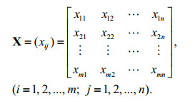 (1)
(1)Calculating the cross product of X and XT:
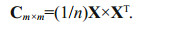 (2)
(2)The eigenvalue (λ1, …, m) and eigenvector Vm×n of C can be obtained:
 (3)
(3)where Λ is an m×m diagonal matrix composed of eigenvalues:
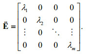 (4)
(4)As the matrix X is the observed value, λ is supposed to be less than zero. Moreover, each non-zero eigenvalue corresponds to a list of eigenvectors, also named EOF. For example, the eigenvector corresponding to eigenvalue λ1 is the first EOF mode, namely the first column of V:
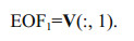 (5)
(5)Projecting EOF to matrix X, the time factor, corresponding to eigenvectors of all space, which is also called the principal component, is determined:
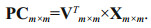 (6)
(6)Each row of the matrix PC is the time factor of the corresponding eigenvector. For a certain EOF mode, the PC represents the temporal significance of its associated spatial function (Monahan et al., 2009).
The standard deviation of principal components reveals the difference in the power of ocean waves at different times (North et al., 1982). When vessel interference exists, the gray level of the vessel can be abnormally high on part of the echo image; the abnormal value appears in the deviation of PC; and energy in the interfered region can raise the noise floor. It will reduce the signal-to-noise ratio (SNR), where the signal is assumed to be the total energy of the wave spectrum caused by sea clutter and the noise is calculated as the energy from the speckle resulting from sea surface roughness (Alpers and Hasselmann, 1982; Chen et al., 2014b). As a result, we could combine the deviation of PC with SNR to supervise the interference efficiently. An empirical analysis provided that, in most cases, a good estimation of the threshold level is 100 with -4 dB for the deviation of PC and SNR, separately. When the deviation of PC is above the threshold level and the value of SNR is below the threshold level, echo images contaminated by vessel interference can be detected. The SNR of the ocean wave spectrum is defined as follows (NietoBorge et al., 2008):
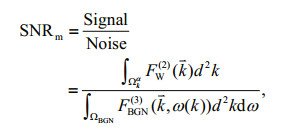 (7)
(7)where FW(2) (k) is the two-dimensional (2-D) signal wave number spectrum, FBGN(3) (k, ω(k)) is the 3-D noise number spectrum, k is the spatial wavenumber, and ω(k) is the angular frequency. The integration domain ΩBGN is the background noise spectral domain, ΩBGN and Ωkα is the signal spectral domain.
4 INTERFERENCE SUPPRESSIONA method based on frequency domain geometric modeling is used to suppress interference. Sea surface image sequences are transformed into the spectral domain by means of a fast Fourier Transform (FFT) to estimate the 3-D spatial wavenumber-frequency spectrum. The signal of linear surface-gravity waves is readily located on a surface in the wave numberfrequency domain defined by the dispersion relation of linear surface-gravity waves. A so-called dispersion shell connects the wave numbers with their corresponding frequency coordinates (Seemann et al., 1999; Gangeskar, 2012). This relationship is revealed in the follow equation
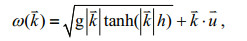 (8)
(8)where ω(k) indicates the angular frequency, g is the gravitational acceleration, h is the water depth, k is the wavenumber and u is the current component (i.e., the sum of the platform velocity and the near-surface current velocity). Next, we introduce a vessel interference suppression method based on the frequency domain geometric model. Because the depth has little effect on the wave dispersion relationship (depth>30 m), the model will work without considering the influence of water depth for the time being. Figure 4 shows the geometric relationship between the spatial wave number and radian frequency in a given direction. For two arbitrary points on the dispersion curve in the 2-D wavenumber-frequency plane, we obtain
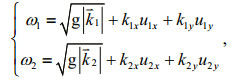 (9)
(9)where ω1 and ω2 are the angular frequency of the two arbitrary points in the radial direction on the dispersion curve, k1=(k1x, k1y), k2=(k2x, k2y) and u1=(u1x, u1y), u2=(u2x, u2y) are the corresponding spatial wavenumber vector and current vector, respectively.

|
| Figure 4 Geometric relationship between the spatial wave number and radian frequency The cone-shaped dispersion shell connects the wavenumbers with their corresponding frequency coordinates; ω1 and ω2 are the angular frequency of two arbitrary points in a radial direction on the dispersion curve. |
In accordance with the dispersion relationship and the geometric configuration (Fig. 4), we obtain
 (10)
(10)assuming that
 (11)
(11)Furthermore, by converting Eq.11 we get
 (12)
(12)From Eq.12 and the geometric model, we know that there is a series of α in a given direction for each point. Moreover, it is constant and can be processed according to the above steps. Hence, for every wavenumber-frequency plane at a given bearing, we can generate a series of curves that satisfy Eq.12. For each curve, we can get the value of energy of each point through the interpolation method (Fig. 5).

|
| Figure 5 For a certain direction, a series of curves satisfying the relationship are determined by the relationship |
As the energy of the echoes that meets the dispersion relation is higher than that of the echoes that diverge from it, we can obtain the echo signal that meets the dispersion curve and around it by comparing the energy values. By repeating the processing procedure above for every bearing and all spectral energy points, based on the geometry model for the linear dispersion relationship for gravity sea surface waves, we obtain an echo signal for different directions. Because the distribution of the spectrum of the vessel echo signal does not meet the gravity wave dispersion relationship, we will get a new unblemished wavenumber-frequency spectrum.
Because the spectrum of a vessel echo signal is always on the low side of the frequency band (Fujikaw and Kojima, 2010; Pestoriza et al., 2010; Pegram et al., 2011), we can further erase some noise and interference by processing the spectrogram with a high-pass filter. After vessel interference suppression on the basis of a frequency domain geometric model and high-pass filtering, we will obtain new unblemished sea surface sequences. The new sea surface sequences can be used to invert for oceanic dynamic parameters. For comparison, a 3-D inverse Fourier transform is performed. The contrast is obvious between the earlier contaminated echo image (Fig. 3) and the image produced after interference suppression (Fig. 6) using this method.

|
| Figure 6 For comparison with the selected region containing vessel interference (Fig. 3) This figure shows the echo image after interference suppression using the method outlined in this paper, with a resolution in the range of 7.5 m. |
By comparing Figs. 3 and 6, we can see that the vessel interference suppression result is improved by using the algorithm. In Fig. 6, we can see the clear stripe information for the ocean wave. By using the vessel interference suppression method based on frequency domain geometric modeling and high-pass filtering, we have efficiently eliminated the interference and produced a less distorted image. In the next section, the characterizations of surface gravity wave parameters, in particular significant wave height (SWH), validate that the use of the suppression method to effectively eliminate the specific kind of interference caused by vessels.
5 RESULT AND DISCUSSIONThe SWH data used for verification of the presented algorithm were obtained from January 1 to 15, 2014, by the Ocean State Measuring and Analyzing Radar type X (OSMAR-X), an X-band wave monitoring radar developed by Wuhan University. The radar is a marine monitoring instrument that has been refitted from navigation radar with an X-bank operating frequency (9 410±30 MHz). The SWH is estimated by using its linearly dependent relationship with the square root of the signal-to-noise ratio (SNR). In ocean-wave observation mode, its performance parameters consist of a maximal detection range of 5 km, a radial range resolution of 7.5 m and the directional resolution of approximately 0.95°. Its antenna dimension is less than 8 ft (2.438 4 m) with a rotation speed of 42 r/min, horizontal polarization, and transmitting power of 12 kW, its pulse width and repetition are 0.07 m s and 3 000 Hz respectively. The radar can run continually for 24 h without a break including data encryption. Additionally, problems with the equipment can be diagnosed and maintained, remotely.
The testing site located in Zhoushan, Zhejiang Province, China, at roughly 29°E, 122°N. The X-band radar station is mounted on top of a hill about 70 m above sea level and 100 m from the shore. To obtain dynamic surveillance and identification information for the vessel, an Automatic Identification System (AIS) was placed at the same location. An in-situ wave buoy (SZF2-1A) was placed 1 000 m away from the radar station at an azimuth of 140°, for comparison. As the buoy archived readings every 30 minutes, the radar was set to the same recording interval. The appearance of the OSMAR-X X-band wave monitoring radar and its testing site are shown in Fig. 7a and b. In Fig. 7b, the blue rectangle is the region selected to retrieve wave parameters.

|
| Figure 7 Appearance (a) and testing site (b) of the OSMAR-X X-band wave monitoring radar The two blue lines denote the FOV of the radar; the radar station itself lies in the little red circle; the blue rectangle is the invention region used to retrieve wave parameters, the blue circle stands for the location of the wave buoy (b). |
Figure 8 shows the comparison of the SWH measured by the buoy with that retrieved from the OSMAR-X X-band wave monitoring radar image sequences, during the period from 1 a.m. to 11 p.m. on January 8 in 2014. The number of data points recorded was 43 and there were three SWH data affected by vessels. We use the SWH calculated from the original contaminated data, and that calculated by the data after interference suppression using the approach mentioned in this paper, to make comparisons with the SWH measured by the buoy. In Fig. 8a, the root-mean-square error and correlation coefficient for the SWH determinations are 0.18 m and 0.85. In Fig. 8b, the corresponding root-mean-square error and correlation coefficient are 0.14 m and 0.91.

|
| Figure 8 Comparison of the SWH measured by the buoy with that retrieved from X-band radar image sequences from 1 a.m. to 11 p.m. on January 8, 2014 a. the red arrows indicate the SWH retrieved from the X-band radar affected by vessels (according to the record of AIS); b. the red arrows indicate the SWH modified by the approach mentioned in this paper. |
Figure 9 shows the comparison of SWH measured by the buoy with that retrieved from the OSMAR-X X-band wave monitoring radar image sequences, from noon to 11 p.m. on January 9, 2014. Of the 23 data points collected, one was affected by vessels. In Fig. 9a, the root-mean-square error and correlation coefficient of the SWH values are 0.15 m and 0.88. In Fig. 9b, the corresponding root-mean-square error and correlation coefficient are 0.12 m and 0.93.

|
| Figure 9 Comparison of the SWH measured by the buoy with that retrieved from X-band radar image sequences from noon to 11 p.m. on January 9, 2014 a. the red arrow indicates the SWH retrieved from the X-band radar affected by vessels (according to the record of AIS); b. the red arrow indicates the SWH modified by the approach mentioned in this paper. |
Table 1 shows the contrast of significant wave height retrieved from original interfered radar image sequences with that measured by the buoy.
As shown in Figs. 8 and 9, and Table 1, our method can readily detect vessel interference. Obviously, the modified inversion results of SWH using the presented algorithm coincide better with the measurements of the buoy than the original value. The root-meansquare error between the significant wave height retrieved from original radar image sequences affected by interference and that measured by the buoy is reduced by 0.25 m (0.471 7 m and 0.219 7 m). Therefore, the method can efficiently mitigate the negative influence of vessel interference, making the inversion results more accurate and stable.
6 CONCLUSIONTo deal with the problem of vessels on the sea surface interfering with ocean wave inversion results, this paper has presented an interference detection and suppression algorithm. The method is less timeconsuming than an inversion of sea state parameters; and therefore is more efficient. Comparison between in situ wave buoy and surface gravity wave parameters, such as significant wave height (SWH) in particular, has proven that the new method can effectively detect and eliminate vessel interference.
The method has produced promising results, although there is still much room for improvement. The following important issues should be considered in future work:
1) different EOF modes should be further studied to obtain more information on wave fields;
2) more statistics should be gathered under various sea states to establish accurate threshold levels for the deviation of PC and SNR;
3) interference data should be collected for use in further performance analysis and to undertake numerical simulations concerning the influence of the sea surface.
| Alpers W, Hasselmann K, 1982. Spectral signal to clutter and thermal noise properties of ocean wave imaging synthetic aperture radars. International Journal of Remote Sensing, 3 (4) : 423 –446. Doi: 10.1080/01431168208948413 |
| An J Q, Huang W M, Gill E W, 2015. A self-adaptive waveletbased algorithm for wave measurement using nautical radar. IEEE Transactions on Geoscience and Remote Sensing, 53 (1) : 567 –577. Doi: 10.1109/TGRS.2014.2325782 |
| Atanassov V, Rosenthal W, Ziemer F, 1985. Removal of ambiguity of two-dimensional power spectra obtained by processing ship radar images of ocean waves. Journal of Geophysical Research, 90 (C1) : 1061 –1067. Doi: 10.1029/JC090iC01p01061 |
| Björnsson H, Venegas S A, 1997. A manual for EOF and SVD analyses of climatic data. CCGCR Rep., 97 (1) : 1 –52. |
| Chen Z B, He Y J, Zhang B, Qiu Z F, 2014a. A new algorithm to retrieve wave parameters from marine X-band radar image sequences. IEEE Transactions on Geoscience and Remote Sensing, 52 (7) : 4083 –4091. Doi: 10.1109/TGRS.2013.2279547 |
| Chen Z B, He Y J, Zhang B, Qiu Z F, 2014b. A new method to retrieve significant wave height from X-band marine radar image sequences. International Journal of Remote Sensing, 35 (11-12) : 4559 –4571. Doi: 10.1080/01431161.2014.916440 |
| Cui L M, He Y J, Shen H, Lü H B, 2010. Measurements of ocean wave and current field using dual polarized X-band radar. Chinese Journal of Oceanology and Limnology, 28 (5) : 1021 –1028. Doi: 10.1007/s00343-010-9056-8 |
| Dankert H, Rosenthal W, 2004. Ocean surface determination from X-band radar-image sequences. Journal of Geophysical Research, 109 (C4) : 1 –11. |
| Fujikaw T, Kojima T. 2010. Radar device and rain/snow area detecting device. Japan, US2010207809 (A1). 2010-08-19. |
| Gangeskar R. 2000. An adaptive method for estimation of wave height based on statistics of sea surface images. In:Proceedings of IEEE International Geoscience and Remote Sensing Symposium. IEEE, Honolulu, HI, USA. 1:255-259. |
| Gangeskar R, 2012. Ocean current estimated from X-band radar sea surface images. IEEE Transactions on Geoscience and Remote Sensing, 40 (4) : 783 –792. |
| Ludeno G, Flampouris S, Lugni C, Soldovieri F, 2014. A novel approach based on marine radar data analysis for highresolution bathymetry map generation. IEEE Transactions on Geoscience and Remote Sensing Letters, 11 (1) : 234 –238. Doi: 10.1109/LGRS.2013.2254107 |
| Lund B, Graber H C, Romeiser R, 2012. Wind retrieval from shipborne nautical X-band radar data. IEEE Transactions on Geoscience and Remote Sensing Letters, 50 (10) : 3800 –3811. Doi: 10.1109/TGRS.2012.2186457 |
| Maa J P Y, Ha H K, 2005. X-band Radar Wave Observation System. College of William and Mary, Herndon, VA, USp.52-53. |
| Monahan A H, Fyfe J C, Ambaum M H P, Stephenson D B, North G R, 2009. Empirical orthogonal functions:the medium is the message. Journal of Climate, 22 (24) : 6501 –6514. Doi: 10.1175/2009JCLI3062.1 |
| Nieto-Borge J C, Hessner K, Jarabo-Amores P, de la MataMoya D, 2008. Signal-to-noise ratio analysis to estimate ocean wave heights from X-band marine radar image time series. IET Radar, Sonar & Navigation, 2 (1) : 35 –41. |
| Nieto-Borge J C, Soares C G, 2000. Analysis of directional wave fields using X-band navigation radar. Coastal Engineering, 40 (4) : 375 –391. Doi: 10.1016/S0378-3839(00)00019-3 |
| North G R, Bell T L, Cahalan R F, Moeng F J, 1982. Sampling errors in the estimation of empirical orthogonal functions. Monthly Weather Review, 110 (7) : 699 –706. Doi: 10.1175/1520-0493(1982)110<0699:SEITEO>2.0.CO;2 |
| Pegram G, Llort X, Sempere-Torres D, 2011. Radar rainfall:separating signal and noise fields to generate meaningful ensembles. Atmospheric Research, 100 (2-3) : 226 –236. Doi: 10.1016/j.atmosres.2010.11.018 |
| Pestoriza V, Nunez A, Marino P, Fontá n F P, 2010. Rain-cell identification and modeling for propagation studies from weather radar images. IEEE Antennas and Propagation Magazine, 52 (5) : 117 –130. Doi: 10.1109/MAP.2010.5687511 |
| Seemann J, Senet C M, Dankert H, Hatten H, Ziemer F. 1999.Radar image sequence analysis of inhomogeneous water surfaces. In:Proceedings of Conference on Applications of Digital Image Processing XXⅡ.SPIE, Denver, CO, USA. |
| Senet C M, Seemann J, Flampouris S, Ziemer F, 2008. Determination of bathymetric and current maps by the method DISC based on the analysis of nautical X-band radar image sequences of the sea surface (November 2007). IEEE Transactions on Geoscience and Remote Sensing Letters, 46 (8) : 2267 –2279. Doi: 10.1109/TGRS.2008.916474 |
| Serafino F, Lugni C, Soldovieri F, 2010. A novel strategy for the surface current determination from marine X-band radar data. IEEE Transactions on Geoscience and Remote Sensing Letters, 7 (2) : 231 –235. Doi: 10.1109/LGRS.2009.2031878 |
| Wu Y Q, Wu X B, Chen F, Ke H Y, 2007. Basic analysis on the extraction of ocean dynamic parameters with an X-band radar. Journal of Remote Sensing, 11 (6) : 817 –825. |
| Young I R, Rosenthal W, Ziemer F, 1985. A three-dimensional analysis of marine radar images for the determination of ocean wave directionality and surface currents. Journal of Geophysical Research, 90 (C1) : 1049 –1059. Doi: 10.1029/JC090iC01p01049 |
| Ziemer F, 1995. An instrument for the survey of the directionality of the ocean wave field. In:Proceedings of.Workshop on Operational Ocean Monitoring Using Surface Based Radars. WMO/IOC Report, Geneva, 32 : 81 –87. |