 2016, Vol. 34
Institute of Oceanology, Chinese Academy of Sciences
Article Information
- YANG Lina(杨丽娜), YUAN Dongliang(袁东亮)
- Absolute geostrophic currents in global tropical oceans
- Chinese Journal of Oceanology and Limnology, 34(6): 1383-1393
- http://dx.doi.org/10.1007/s00343-016-5092-3
Article History
- Received Mar. 26, 2015
- accepted for publication Jun. 9, 2015
- accepted in principle Sep. 30, 2015


2 University of Chinese Academy of Sciences, Beijing 100049, China;
3 Key Laboratory of Ocean Circulation and Waves, Chinese Academy of Sciences, Qingdao 266071, China;
4 Qingdao Collaborative Innovation Center of Marine Science and Technology, Qingdao 266003, China
Since Sverdrup (1947) introduced the dynamic framework of ocean circulation when studying equatorial currents in the eastern Pacific Ocean, this theory has become the cornerstone of modern oceanography. The analysis of the relationship between wind stress and prevailing baroclinic currents has been extended to other studies (Leetmaa et al., 1977 ; Meyers, 1980 ; Wunsch and Roemmich, 1985 ; Böning et al., 1991 ; Schmitz et al., 1992 ; Hautala et al., 1994). Their results suggest that the theory does not apply to the subtropical northwestern Atlantic Ocean or tropical northwestern Pacific Ocean. However, the lack of sufficient measurements, especially at basin scale, hinders the acquisition of accurate ocean circulation datasets. Accordingly, the validity of the theory has not been examined extensively, and efforts in this direction must be continued.
Fortunately, the aforementioned dilemma has been greatly ameliorated by the advent of the Argo project, which for the first time allowed continuous monitoring of temperature and salinity of the upper 2 000 m of the global oceans. Wunsch (2011) examined the Sverdrup theory based on an assimilated global ocean dataset, concluding that failure of a basin-wide integral test does not preclude the possibility of the accuracy of the Sverdrup balance at individual points, and his results showed that the linear dynamics have quantitative skill in depicting the observed ocean circulation across much of the subtropical and lower latitudes (about 40% of the global oceans). Based on P-vector AGCs from gridded Argo profiling data, Zhang et al.(2013) and Yuan et al.(2014) identified significant discrepancies in the North Pacific, immediately north and south of the bifurcation latitude of the North Equatorial Current west of the dateline and in the recirculation area of the Kuroshio and its extension. To evaluate the Sverdrup theory, Gray and Riser (2014) calculated velocities at the reference level of 900 db and global absolute geostrophic velocity using trajectory data and temperature and salinity profiles from the Argo floats. Their results show that observed transport agrees well with predictions based on wind stress over large areas, primarily in the tropics and subtropics.
Despite these groundbreaking achievements, deficiencies remain. Analyses have suggested that neglect of bottom relief (known as the joint effect of baroclinicity and relief of the bottom or JEBAR) is one of the principal restrictions of the Sverdrup circulation theory (Marchuk et al., 1973 ; Polonsky, 2015), and few investigations made quantitative calculations of this effect. In addition, the analysis of Wunsch (2011) is based on output of an ocean model, but there is no way of determining to what extent the model depicts the observations. The geostrophic analysis of Gray and Riser (2014) does not conserve mass and potential vorticity in general, and Yuan et al.(2014) evaluated the Sverdrup theory only in the North Pacific. Therefore, the present study extends the Sverdrup dynamics analysis to the world tropical oceans, taking the JEBAR into account.
Except for the parking-depth method of Gray and Riser (2014), there are some traditional inverse methods to calculate AGCs, including the β-spiral (Stommel and Schott, 1977), box inverse (Wunsch, 1978), Bernoulli (Killworth, 1986) and P-vector (Chu, 1995, 2006) methods. The four inverse methods have the same order of dynamical sophistication (geostrophy, hydrostatic equilibrium and density conservation) but different treatments.
Substantial noise is introduced by the use of second partial differentials of water density in the β-spiral method. The underdetermined system naturally leads to substantial uncertainty in the box inverse method. The Bernoulli method, which is designed for a sparse field, turns into the β-spiral method when data are of high resolution. Dynamically, the P-vector method is equivalent to the β-spiral method under the Boussinesq and geostrophic approximation (Yuan et al., 2014), but use of only the first order derivatives of density field greatly improves the accuracy of solutions. Therefore, in the present study, the P-vector method was used to calculate the global AGCs and, in light of the greater uncertainties of AGCs at high latitudes, the oceans between 30°S and 30°N were studied.
The outline of this paper is as follows. The data and methods of AGC calculation are described in Section 2. In Section 3, the calculated AGCs are compared with altimeter, OSCAR and global moored current meter data, based on which the Sverdrup theory is evaluated. After presenting a discussion of sensitivity and errors of the analysis in Section 4, key results are summarized in Section 5.
2 DATA AND METHOD 2.1 DataGridded Argo temperature and salinity data (http:// www.argo.ucsd.edu/Gridded_fields.html) from January 2004 to December 2012, with 1°×1° horizontal resolution and 58 vertical layers in the top 2 000 m of the ocean, were provided by the Scripps Institution of Oceanography and used to calculate the AGCs (Roemmich and Gilson, 2009).
The wind data used to calculate surface Ekman velocity and Sverdrup transport are National Centers Environmental Prediction / National Center for Atmospheric Research (NCEP/NCAR) reanalysis monthly means (http://www.esrl.noaa.gov/psd/data/gridded/data.ncep.reanalysis.derived.surfaceflux.html) from January 1948 to present, with spatial resolution 2.5° longitude×2.5° latitude (Kalnay et al., 1996). In addition, the European Centre for Medium-Range Weather Forecasts Interim Reanalysis (ERA-Interim) global atmospheric reanalysis (http://apps.ecmwf.int/datasets/data/interim-full-moda/) from 1979 to present, with spatial resolution 0.75°×0.75°, was used to compute Sverdrup transport for comparison.
Maps of Absolute Dynamic Topography (ftp.aviso. oceanobs.com) data used to calculate surface geostrophic currents for comparison are produced by the Data Unification and Altimeter Combination System and distributed by the Archiving, Validation and Interpretation of Satellite Oceanographic project. This gridded product has spatial resolution 1/3°×1/3° and is based on two missions at most, i.e., Jason-2/ AltiKa or Jason-2/Cryosat-2 or Jason-2/Envisat, or Jason-1/Envisat or Topex/Poseidon / ERS, with the same ground track. Thus, the product is homogeneous throughout the available time period thanks to stable sampling. But it must be kept in mind that the data might not be of the best possible quality despite the great stability.
Ocean Surface Current Analysis-Real time (OSCAR) currents (http://www.oscar.noaa.gov/datadisplay/oscar_datadownload.php) on a 1° longitude×1° latitude grid are estimated using satellite-derived sea level and wind stress fields. Monthly mean currents are used to validate the P-vector currents at the surface.
Daily 10-m depth current meter data (http://www.pmel.noaa.gov/tao/data_deliv/deliv.html), also used to validate the P-vector currents, are from the Global Tropical Moored Array, a multinational effort to provide datain real-time for climate research. The array includes the Tropical Atmosphere Ocean / Triangle Trans-Ocean Buoy Network in the Pacific, Prediction and Research Moored Array in the Atlantic, and Research Moored Array for African-Asian- Australian Monsoon Analysis and Prediction in the Indian Ocean.
2.2 P-vector method to calculate AGCsAGCs are calculated based on the P-vector method using the intersections of isopycnal and potential vorticity surfaces (known as the P-vector), to determine the direction of geostrophic currents. The thermal wind relationship is then used to calculate magnitudes of the currents using least-squares fitting of the vertical layers (Chu, 1995, 2006). Because the conservation of density and potential vorticity does not generally hold in the upper mixed layer of the ocean, the procedure followed that of Yuan et al.(2014). P-vector currents between 800 and 2 000 db were constructed, and then currents above 800 db were determined through dynamic height calculation, using P-vector velocity at 800 db as the reference velocity. Experiments have shown that magnitudes and structure of AGCs are generally insensitive to the choice of the aforementioned depth ranges, as long as the P-vector calculation is for substantially below the surface mixed layer. Ageostrophy is considerable near the equator owing to the very small Coriolis force, so the geostrophic calculation was applied outside regions of 4°S-4°N.
2.3 Surface Ekman currentsEkman velocity is estimated using the method of Lagerloef et al.(1999), which defined a two-parameter Ekman model between 25°S and 25°N.
 (1)
(1)where h =32.5 m is the scaling thickness, r =2.15×10⁻⁴ m/s the drag coefficient representing the vertical viscosity terms, τ =τ x + iτ y the zonal and meridional wind stress, and 
The foundation of the parametric test of significance is the number of degrees of freedom (DOF), which is often estimated based on lagged auto-correlation coefficients. Consider a time series (ai, i =1, …, NT) sampled at regular interval Δ t. NT is generally not an appropriate estimate of the number of DOF because of serial coherence. In this study, the number of DOF was estimated according to the equation of Bretherton et al.(1999) :
 (2)
(2)where ν is the number of DOF, r (Δ t) is the autocorrelation coefficient, and NT is the sampling number.
The standard error SE of a time average as an unbiased estimate of the climatology decreases asymptotically as the inverse of the square root of record length (Leith, 1973). Thus, if there is a sample of ν independent values with standard deviation σ, then SE =σ /$\sqrt v $.
2.5 Sverdrup balanceSverdrup (1947) introduced a relationship for the distribution of vertically-integrated baroclinic geostrophic transport to wind stress under the assumption of a maximum depth H in the ocean, beyond which the horizontal and vertical velocities vanish. Following the definition of Hautala et al.(1994), the Sverdrup balance is computed as
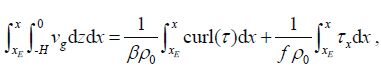 (3)
(3)where xE represents the eastern boundary, v g the meridional AGCs, β =d f /d y the meridional gradient of the Coriolis parameter, ρ0 water density, and (τ x, τ y) the wind stress components. Other notation is standard. The first term on the right side of Eq.3 is known as the Sverdrup transport, and the second designates surface Ekman transport. Collectively, these two terms are called S−E transport for short, and can be computed based on surface wind stress only.
3 RESULT 3.1 P-vector geostrophic currents and error estimatesGlobal AGCs between 30°S and 30°N at the sea surface calculated using the P-vector method are shown in Fig. 1a. From this, surface equatorial currents and subtropical gyres are easily identified, consistent with the current depiction of the ocean general circulation. Magnitudes of currents at depth (e.g., 1 000 db (Fig. 1b) and 1 975 db (Fig. 1c)) can reach a few centimeters per second, which means that the traditional dynamic height method may cause relatively large errors in velocity and corresponding transport.

|
| Figure 1 Mean AGCs from January 2004 to December 2012 at the surface (a), 1 000 db (b), and 1 975 db (c) calculated using P-vector (between 800 and 1 975 db) and dynamic height (above 800 db) methods, based on gridded Argo temperature and salinity data |
The number of DOF for zonal velocity (Fig. 2a) decreased more than that of meridional velocity (Fig. 2b) over most areas, owing to the strong seasonal cycle of zonal geostrophic currents. The number of DOF for zonal velocity is generally greater than 50, while that for meridional velocity reaches 100. For the water column above 800 db, the horizontal velocity in each layer L k may accumulate the errors of all layers below L k with use of the dynamic height method, which does not occur in the water column below that level. Given this, we believe that the error of AGCs is mainly from two sources. One is from time dependence below 800 db, and the other is based on standard deviation of the density above 800 db combined with the thermal wind relationship. Figure 2c and d shows the upper limit of standard error of zonal and meridional velocity, respectively, with error of the zonal AGCs < 2 cm/s and that of the meridional AGCs < 1 cm/s over most of the oceans. In equatorial current regions, larger uncertainties of zonal velocity correspond to the strong seasonal cycle, and can be reduced remarkably by using a nine-year average.

|
| Figure 2 Number of DOF for zonal (a) and meridional (b) AGCs from January 2004 to December 2012 Contour interval is 5. Standard error of zonal (c) and meridional (d) AGCs at sea surface. Contour interval is 0.5 cm/s. |
The co-relationship (Fig. 3a, b) and root mean square (RMS) differences (Fig. 3c, d) were compared between surface currents from P-vector AGCs and altimeter geostrophic currents. Areas with correlation coefficients >0.19(95% significance level corresponding to 107 DOF) occupy a large portion of global tropical ocean basins. The number of DOF distribution suggests that the significance test remained relatively unchanged. For zonal velocity, the coefficients are sufficiently large, in spite of the relatively small DOF (e.g., in areas of the westward equatorial currents). Correlation coefficients where the DOF is small originally failed to pass the significance test. For meridional velocity, the DOF barely decreased. Generally, the co-relationship is poor in areas with sparse distribution of Argo floats, because the altimeter data with better spatial resolution can readily track mesoscale eddies, whereas the smoothed Argo data cannot. However, the variation can be filtered by taking the average of the time series.

|
| Figure 3 Correlation coefficients (a, b) and RMS differences (c, d) between surface AGCs and altimeter geostrophic currents from January 2004 to December 2012 Upper two panels show zonal velocity and lower two meridional velocity. In panels a and b, colored areas represent values > 0.19, and contour interval is 0.075. In panels c and d, contour interval is 2 cm/s. |
RMS differences of the zonal and meridional currents were <4 cm/s over most of the oceans, within the error bars of the altimeter geostrophic currents evaluated by Rio and Hernandez (2004). Larger differences were found near the equator with active eddies, which are not resolved well by the Argo data. We also compared the surface AGCs and OSCAR currents (with the surface Ekman currents subtracted), giving nearly the same results. The comparisons suggest the validity of the P-vector AGCs, which can be used for further studies of large-scale ocean circulation.
The surface P-vector AGCs were also compared with moored current meter measurements at 10-m depth in the Atlantic, Pacific and Indian oceans. Correlation coefficients (values outside parentheses) and RMS differences (values inside parentheses) of the comparisons are listed in Table 1. In general, the zonal AGCs are in good agreement with the mooring measurements. All correlation coefficients are above the 95% significance level except for stations at (12°N, 23°W) and (10°S, 10°E), where the current meter time series are short. For meridional currents, the correlation is low for stations at (15°N, 38°W), (9°N, 140°W), (8°N, 156°E), (5°S, 156°E), and (8°S, 125°W). This is attributed to the short time series of the current meter data, generally weak currents in the meridional direction, and inaccuracies in the surface Ekman velocity calculation. Geostrophic current estimates of the satellite altimeter contain sizable errors, especially for weak meridional currents, because of finite differencing of sea level and its errors (~2 cm). Thus, the P-vector AGCs can be used to evaluate the Sverdrup theory in the world oceans at lower latitudes.

|
Based on the mean AGCs from January 2004 to December 2012, the Sverdrup circulation theory was evaluated over the global tropical oceans. Figure 4a shows zonally and vertically integrated meridional geostrophic transport in the upper 2 000 m from the eastern boundary of the ocean basin. The integrated AGC transport is also the stream function of the vertically integrated geostrophic circulation. It shows prominent subtropical gyres in each ocean basin of both hemispheres except in the North Indian Ocean, where the mean ocean circulation is weak because of the monsoon climate. The AGCs and associated transport are independent of the level of no motion and are thus more objective than those from the dynamic height calculations. The stream function near Western Australia was not zero, and is calculated by d ψ = u d y - v d x as follows. Assuming that the stream function along the western boundary of Java Island is zero, we integrate the depth-integrated AGCs westward first, then integrate the zonal velocity southward along 100°E and finally integrate the meridional velocity eastward and westward to obtain the stream function over the entire tropical South Indian Ocean.
In comparison with the geostrophic stream function, S−E transport (Fig. 4b) derived from the mean NCEP wind stress during the same period as the AGCs, based on the drag coefficient of Garratt (1977), reveals subtropical gyres that are more zonally aligned and of different latitudinal ranges than the geostrophic stream function. Here, S−E transports along the Western Australia coast were set to the same values as the geostrophic stream function to make their differences there zero, thereby avoiding the accumulation of errors from the eastern boundary of the ocean basin. The difference between the AGC and S−E transports is shown in Fig. 4c. Significant non-Sverdrup transport is identified in the subtropical western ocean basins, the Subtropical Counter Current (STCC) areas, and between the Equatorial current and the Equatorial Counter Current. The presence of this type of non-Sverdrup circulation in the North Pacific Ocean has been discussed in detail by Yuan et al.(2014), who suggested nonlinear effects of the ocean circulation as the reason for the discrepancies. We extended our examination to the global tropical oceans, as discussed in the following section.

|
| Figure 4 Mean transport of meridional AGCs above 2000 m (a); S−E transport derived from mean NCEP wind stress (2004- 2012) based on drag coefficient of Garratt (1977) (b); difference between AGC and S−E transports (c) Contour interval is 5 Sv. Gray shading indicates negative values. |
To examine whether the discrepancy between meridional geostrophic transport and S−E transport (i.e., the non-Sverdrup transport) is robust, errors of the former transport were estimated. The error bar is extended unreasonably if one directly accumulates the estimated errors of the AGCs (shown in Section 3.1), because those errors will offset each other while integrating westward. Given that fact, the standard deviation of the time series (January 2004 to December 2012) of monthly geostrophic transports was used. The minimum DOFs at each latitude in each ocean basin were selected to estimate the standard error (Fig. 5), which was <1 Sv in most ocean basins. Relatively large errors (essentially <3 Sv) are mainly within 10°S-10°N in the Pacific and Indian Oceans, still much less than the discrepancies there. This suggests that errors of the meridional AGC transports do not alter the substantial discrepancies between the AGC and S−E transports.

|
| Figure 5 Error estimates of meridional geostrophic transport based on time series of monthly AGC transports and estimated DOF at each latitude Contour interval is 0.5 Sv. Gray shading indicates values <1 Sv. |
Examination of the robustness of the discrepancies was done using various lower limits H of the vertical integration, wind products, and drag coefficients. Figure 6 shows the comparison. In panels a and b, the only thing that differentiates them from Fig. 4c is that the vertically integrated non-Sverdrup transports are above the 27.2σθ and 27.5σθ isopycnic surfaces, respectively. Nearly the same discrepancy pattern implies insensitivity of the calculation to the H of the vertical integration. Figure 6c and d, using the same H (σθ =27.5) and wind product (ECMWF) but different drag coefficients (Garratt (1977) for c and Large and Pond (1981) for d), show nearly the same results, which means that the discrepancy is insensitive to the method of calculating wind stress. With the same H of vertical integration (σθ =27.5) and drag coefficient (Garratt, 1977), Fig. 6b and c compare different wind products. As seen, despite some differences between the results of different wind products (NCEP and ECMWF), the main structure of the non-Sverdrup gyre, which is prominent across 5°-10° in both hemispheres, between the equatorial current and STCC, and in the subtropical western basins, is constant. The main differences between Fig. 6b and c are across 10°-20°N and 5°-10°S in the Pacific. The discrepancy from the ECMWF wind stress appears smaller than that from the NCEP wind stress. Comparison between the two wind products (figure not shown) shows that the ECMWF wind stress is smaller and smoother than that of NCEP, suggesting that a more accurate analysis of the Sverdrup circulation theory requires a more accurate wind product. The identified discrepancy from simple linear Sverdrup dynamics is robust, in spite of the aforementioned differences.
4.3 Joint effect of baroclinicity and relief of the bottom (JEBAR)The magnitude of vertical velocity at H of the vertical integration of the geostrophic currents is estimated by considering H as the depth of isopycnic surfaces (here, 27.5σθ is selected), using
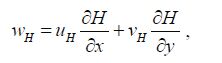 (4)
(4)where wH, uH and vH, respectively, represent vertical velocity, zonal velocity and meridional velocity at depth H. Then, the meridional transport caused by the JEBAR is assessed by
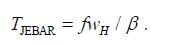 (5)
(5)From Fig. 7a, the zonally integrated TJEBAR has relatively large magnitudes poleward of the confluence of the equatorial current and STCC (except the eastern boundary), where the gradient of horizontal velocity at H is large. After considering TJEBAR, the discrepancy between the geostrophic transport and the S−E transport (Fig. 6b) is modified (Fig. 7b). The modified differences over 20°-30°S of each ocean basin increase, and it is speculated that except for the surface wind curl and JEBAR, mesoscale eddy nonlinearity is important there. Previous studies (Qiu, 1999 ; Jia and Wu, 2011 ; Chang et al., 2015) suggest strong eddy activity in the STCC and near the western boundary. Although the time-mean ocean circulation transports fluid as a conveyor belt, fluid parcels can be trapped within eddy cores and transported discretely by migrating mesoscale eddies (Zhang et al., 2014). Chang et al.(2015) analyzed the effect of STCC eddies on the upstream Kuroshio, finding that the Kuroshio transport is strengthened by the wind during eddy-rich years relative to eddy-poor years, being caused by mass convergence and divergence. The effect of eddies during eddy-rich years cannot offset that during eddy-poor years, so mesoscale eddies can influence time-mean ocean circulation transports. In addition, eddies in the upstream Kuroshio can propagate downstream, thereby affecting the downstream Kuroshio. The detailed dynamics of this requires further study. TJEBAR in the Northern Hemisphere is weaker, except to the east of the Florida, where the modified difference decreases greatly, suggesting the importance of JEBAR there. In the remaining areas, TJEBAR is negligible and the circulation is presumed to be dominated by the β effect, surface wind curl, and nonlinear advection.

|
| Figure 6 a. vertically-integrated non-Sverdrup function above the 27.2 isopycnic surface and NCEP wind stress over 2004-2012 using drag coefficient of Garratt (1977) ; b. as in (a), but above the 27.5 isopycnic surface; c. as in (b), but based on ERA-Interim wind stress; d. as in (c), but using drag coefficient of Large and Pond (1981) Gray shading indicates negative values. Contour interval is 5 Sv. |

|
| Figure 7 a. meridional transport caused by JEBAR. Contour interval is 3 Sv; b. difference between geostrophic (above 27.5 isopycnic surface) and S−E (NCEP; Garratt, 1977) transport, after considering JEBAR. Contour interval is 5 Sv Gray shaded areas indicate negative values. Units are Sv. |
A set of monthly mean AGCs in the global tropical oceans were calculated based on gridded Argo temperature and salinity profiles from January 2004 to December 2012, using the P-vector method. The AGCs show relatively good agreement with altimeter currents, OSCAR currents, and moored current-meter data, suggesting the validity of the geostrophic currents. The latter currents may thus be used to study the general circulation in the global tropical oceans. Accuracy of the Sverdrup balance was then assessed by comparing meridional geostrophic transport with S−E transport. Discrepancies in each ocean basin share the feature that the Sverdrup balance is deficient in describing geostrophic transport in the western subtropical oceans, STCC, and between the equatorial current and Equatorial Counter Current. Calculations showed that the discrepancies are insensitive to errors of AGC transports, lower limits of the vertical integration, drag coefficients of the wind stress calculation, and various wind products. This suggests that errors of the wind stress calculation and AGC transports, and vertical integration, cannot explain the deviation from Sverdrup balance. Combined with the JEBAR calculation, it is speculated that in the Southern Hemisphere, the surface wind curl, JEBAR and mesoscale eddy nonlinearity combined regulate the STCC and western boundary current. In the Northern Hemisphere where the JEBAR is generally small, the circulation is presumed to be dominated by the surface wind curl and nonlinear advection in the STCC and between the equatorial current and Equatorial Counter Current of the western ocean basin. The exception to this is the area east of Florida, where the JEBAR is important. These results suggest that the linear Sverdrup dynamics may be deficient, even in the interior of the ocean basin.
| Böning C W, Döscher R, Isemer H J, 1991. Monthly mean wind stress and Sverdrup transports in the North Atlantic:a comparison of the Hellerman-Rosenstein and IsemerHasse climatologies. J. Phys. Oceanogr., 21 (2) : 221 –235. Doi: 10.1175/1520-0485(1991)021<0221:MMWSAS>2.0.CO;2 |
| Bretherton C S, Widmann M, Dymnikov V P, et al, 1999. The effective number of spatial degrees of freedom of a timevarying field. J. Clim., 12 (7) : 1 990 –2 009. Doi: 10.1175/1520-0442(1999)012<1990:TENOSD>2.0.CO;2 |
| Chang Y L, Miyazawa Y, Guo X Y, 2015. Effects of the STCC eddies on the Kuroshio based on the 20-year JCOPE2 reanalysis results. Prog. Oceanogr., 135 : 64 –76. Doi: 10.1016/j.pocean.2015.04.006 |
| Chu P C, 1995. P-vector method for determining absolute velocity from hydrographic data. Mar. Technol. Soc. J., 29 (3) : 3 –14. |
| Chu P C. 2006. P-vector Inverse Method. Springer, Berlin Heidelberg. 605p. |
| Garratt J R, 1977. Review of drag coefficients over oceans and continents. Mon. Wea. Rev., 105 (7) : 915 –929. Doi: 10.1175/1520-0493(1977)105<0915:RODCOO>2.0.CO;2 |
| Gray A R, Riser S C, 2014. A global analysis of sverdrup balance using absolute geostrophic velocities from argo. J. Phys. Oceanogr., 44 (4) : 1 213 –1 229. Doi: 10.1175/JPO-D-12-0206.1 |
| Hautala S L, Roemmich D H, Schmilz Jr W J, 1994. Is the north pacific in sverdrup balance along 24°N? J. Geophys.Res., 99 (C8) : 16 041 –16 052. Doi: 10.1029/94JC01084 |
| Jia F, Wu L X, Qiu B, 2011. Seasonal modulation of eddy kinetic energy and its formation mechanism in the southeast Indian Ocean. J. Phys. Oceanogr., 41 (4) : 657 –665. Doi: 10.1175/2010JPO4436.1 |
| Kalnay E, Kanamitsu M, Kistler R, et al, 1996. The NCEP/NCAR 40-year reanalysis project. Bull. Amer. Meteor.Soc., 77 (3) : 437 –471. Doi: 10.1175/1520-0477(1996)077<0437:TNYRP>2.0.CO;2 |
| Killworth P D, 1986. A Bernoulli inverse method for determining the ocean circulation. J. Phys. Oceanogr., 16 (12) : 2 031 –2 051. Doi: 10.1175/1520-0485(1986)016<2031:ABIMFD>2.0.CO;2 |
| Lagerloef G S E, Mitchum G T, Lukas R B, Niiler P P, 1999. J. Geophy. Res.. 23 313-23 326. |
| Large W G, Pond S, 1981. Open ocean momentum flux measurements in moderate to strong winds. J. Phys.Oceanogr., 11 (3) : 324 –336. Doi: 10.1175/1520-0485(1981)011<0324:OOMFMI>2.0.CO;2 |
| Leetmaa A, Niiler P, Stommel H, 1977. Does the Sverdrup relation account for the mid-Atlantic circulation? J. Mar.Res., 35 : 1 –10. |
| Leith C E, 1973. The standard error of time-average estimates of climatic means. J. Appl. Meteor., 12 (6) : 1 066 –1 069. Doi: 10.1175/1520-0450(1973)012<1066:TSEOTA>2.0.CO;2 |
| Marchuk G I, Sarkisian A J, Kochergin V P, 1973. Calculations of flows in a baroclinic ocean:numerical methods and results. Geophys., Fluid Dyn., 5 (1) : 89 –99. Doi: 10.1080/03091927308236109 |
| Meyers G, 1980. Do Sverdrup transports account for the Pacific North Equatorial Countercurrent? J. Geophys.Res., 85 (C2) : 1 073 –1 075. Doi: 10.1029/JC085iC02p01073 |
| Polonsky A, 2015. Comments on "a global analysis of sverdrup balance using absolute geostrophic velocities from argo". J. Phys. Oceanogr., 45 (5) : 1 446 –1 448. Doi: 10.1175/JPO-D-14-0127.1 |
| Qiu B, 1999. Seasonal eddy field modulation of the North Pacific Subtropical Countercurrent:TOPEX/Poseidon observations and theory. J. Phys. Oceanogr., 29 (10) : 2 471 –2 486. Doi: 10.1175/1520-0485(1999)029<2471:SEFMOT>2.0.CO;2 |
| Rio M H, Hernandez F, 2004. A mean dynamic topography computed over the world ocean from altimetry, in situ measurements, and a geoid model. J. Geophys.Res., 109 (C12) : C12302 . Doi: 10.1029/2003JC002226 |
| Roemmich D, Gilson J, 2009. The 2004-2008 mean and annual cycle of temperature, salinity, and steric height in the global ocean from the Argo program. Prog. Oceanogr., 82 (2) : 81 –100. Doi: 10.1016/j.pocean.2009.03.004 |
| Schmitz W J, Thompson J D, Luyten J R, 1992. The Sverdrup circulation for the Atlantic along 24°N. J. Geophys. Res., 97 (C5) : 7 251 –7 256. Doi: 10.1029/92JC00417 |
| Stommel H, Schott F, 1977. The beta spiral and the determination of the absolute velocity field from hydrographic station data. Deep Sea Res., 24 (3) : 325 –329. Doi: 10.1016/0146-6291(77)93000-4 |
| Sverdrup H U, 1947. Wind-driven currents in a baroclinic ocean; with application to the equatorial currents of the eastern Pacific. Proc. Natl. Acad. Sci. USA, 33 (11) : 318 –326. Doi: 10.1073/pnas.33.11.318 |
| Wunsch C, Roemmich D, 1985. Is the north atlantic in sverdrup balance? J. Phys. Oceanogr., 15 (12) : 1 876 –1 880. Doi: 10.1175/1520-0485(1985)015<1876:ITNAIS>2.0.CO;2 |
| Wunsch C, 1978. The North Atlantic general circulation west of 50°W determined by inverse methods. Rev. Geophys., 16 (4) : 583 –620. Doi: 10.1029/RG016i004p00583 |
| Wunsch C, 2011. The decadal mean ocean circulation and Sverdrup balance. J. Mar. Res., 69 (2-3) : 417 –434. |
| Yuan D L, Zhang Z C, Chu P C, Dewar W K, 2014. Geostrophic circulation in the tropical north pacific ocean based on argo profiles. J. Phys. Oceanogr., 44 (2) : 558 –575. Doi: 10.1175/JPO-D-12-0230.1 |
| Zhang Z C, Yuan D L, Chu P C, 2013. Geostrophic meridional transport in tropical northwest Pacific based on Argo profiles. Chin. J. Oceanol. Limnol., 31 (3) : 656 –664. Doi: 10.1007/s00343-013-2169-0 |
| Zhang Z G, Wang W, Qiu B, 2014. Oceanic mass transport by mesoscale eddies. Science, 345 (6194) : 322 –324. Doi: 10.1126/science.1252418 |