 2017, Vol. 35
Institute of Oceanology, Chinese Academy of Sciences
Article Information
- YANG Xianping(杨宪平), SOKOLETSKY Leonid, WEI Xiaodao(魏小岛), SHEN Fang(沈芳)
- Suspended sediment concentration mapping based on the MODIS satellite imagery in the East China inland, estuarine, and coastal waters
- Chinese Journal of Oceanology and Limnology, 35(1): 39-60
- http://dx.doi.org/10.1007/s00343-016-5060-y
Article History
- Received Mar. 3, 2015
- accepted for publication Jul. 13, 2015
- accepted in principle Dec. 25, 2015


Coastal ecosystems are among the most productive ecosystems in the world, playing a major role in water, carbon, nitrogen, and phosphorous cycles between land and sea. Furthermore, coastal regions are home to about two thirds of the world's population (Cracknell, 1999). The suspended sediment concentration (SSC) and chlorophyll a (Chl) concentration are among the most important water quality components. They directly affect light distribution and, therefore, the ocean's primary production and growth of ocean agriculture (Gordon and McCluney, 1975). SSC data are essential for understanding water quality because suspended sediments can control the transport of nutrients, reduction of light penetration and fluxes of metals, radio-nuclides and organic micropollutants (Ouillon et al., 2004 ; Wang et al., 2009). Besides, degradation of water quality due to elevated SSC also affects aquatic organisms and has become a major global environmental problem (Schiebe et al., 1992).
The environment of East China Sea (ECS) has been impacted by huge stresses from anthropogenic activities and population growth in the Changjiang (Yangtze) River drainage basin and adjacent areas along the coasts. Improper use of natural resources and short-term economic objectives have resulted in severe environmental degradation in a fairly short time, and the degradation has now reached a level where the health and well being of the coastal populations are threatened (Li and Dag, 2004).
The concentrations of SSC and Chl in the water strongly influence the turbidity and color of water bodies (Harrington Jr et al., 1992 ; Pozdnyakov et al., 1998). In recent years, there is an increasing interest in satellite retrieval of water substances concentrations for optically complex Case 2 coastal waters. For this aim, numerous different algorithms based on surface reflectance were suggested. However, there still exists an insufficient understanding among the aquatic optics community as to the advantages and disadvantages of such algorithms, especially in the case of extremely turbid waters. Thus, it seems important to develop new SSC retrieval algorithms, which are adapted for turbid waters with a wide range SSC and Chl, to cover real situations in the Chinese inland, coastal, and estuarine waters.
Most of the present remote-sensing algorithms for SSC retrieval are based on using so-called spectral remote-sensing reflectance Rrs (λ) or some spectral combinations of this parameter (Ma and Dai, 2005 ; Zhou et al., 2006 ; Ouillon et al., 2008). This parameter is determined for the plane just above the air-water surface as the ratio of the spectral water-leaving radiance Lw (λ) to the spectral incident irradiance Ed (λ). Thus, an accurate determination of this parameter from the marine radiometric measurements is an important issue. However, there is still no consensus in the aquatic optics community about the standard method for Rrs (λ) determination. We will analyze different approaches to estimation of Rrs (λ) and a related parameter, the sky radiance spectral reflectance ρsky (λ).
In this paper three important issues necessary for satellite water quality remote sensing are considered: 1) an atmospheric correction method (Section 2.2); 2) radiometric models for Rrs (λ) and ρsky (λ)(Section 2.3); and 3) SSC versus Rrs (λ) models (section 2.4). We have solved these problems in a connection to the East China natural waters [mainly Changjiang River estuary (YRE) and its adjacent coastal area (ACA)], and generated several SSC maps for the region in 2008-2013.
2 MODELING APPROACH 2.1 Study area, ground and remote-sensing dataThe East China inland, coastal and estuarine waters are characterized by suspended sediments with concentrations varied from ~10-100 g/m3 in the ECS waters, up to ~2 500 g/m3 in Changjiang River mouth and up to ~5 000 g/m3 in the Subei Bank of the Yellow Sea and Hangzhou Bay (Shen et al., 2010a, 2010b, 2013, 2014 ; He et al., 2012, 2013 ; Sokoletsky et al., 2014a).
Three databases were used in the present work for model development and validation purposes: 1) laboratory tank measurements performed in July 2006(118 samples), when the sediment samples were collected in Changjiang and Huanghe (Yellow) River estuaries (Shen et al., 2010a); and 2) two series of in situ measurements performed in May 2011(19 samples) and in February-March 2014(94 samples) in the estuary of the Changjiang River and coastal zone of the East China Sea. However, the simultaneous field measurements of Chl, SSC, and the spectral radiometric fluxes were made only during February 17 to March 10, 2014 scientific cruise.
Figure 1 shows the locations, including the Changjiang River and its estuary, Hangzhou Bay, Taihu Lake, Yellow Sea, and the ACA of the ECS. The wind speed W was measured by the Handheld anemometer and ranged from 0.5 to 8.0 m/s at average value (±standard deviation) of 2.8(±1.5) m/s. The solar zenith angle (SZA)θ0 was estimated from the geographical coordinates of the sites and the times of measurements by the standard methods with the small modifications as described in Sokoletsky et al.(2011). The range of variability for θ0 was 35 to 85 deg at average value (±standard deviation) of 54(±13) deg.

|
| Figure 1 Map of the eastern Chinese waters The circles show the locations of the field measurements. |
Methods of Chl and SSC measurements were described in Shen et al.(2010c) and Sokoletsky and Shen (2014), respectively. The Chl observations were performed only during February 17 to March 10, 2014(93 samples) with the average and standard deviation values for subsurface samples of 2.6(±1.2) mg/m3. The similar statistical measures for all 191 subsurface SSC samples are 243(±539) g/m3. Subsurface values of Chl and SSC during February 17 to March 10, 2014 varied in the ranges from 0.2 to 6.7 mg/m3 and 3.9 to 475 g/m3, respectively (Fig. 2). Values of SSC varied from 3.9-24(with the mean of 10 g/m3), 8.1-70(with the mean of 25 g/m3), and 61- 475(with average of 201 g/m3) g/m3 in moderate, turbid, and ultra-turbid waters, correspondingly; however, Chl values do not reveal any correlation with the water types (Fig. 2). A statistical analysis shows that the relation between Chl and SSC is very weak with the determination coefficient R2 =0.017 and two-tailed significance level P =0.21.

|
| Figure 2 Chlorophyll a and SSC values derived from the subsurface field measurements in the East China coastal area during February 17 to March 10, 2014 The green, yellow, and red symbols correspond to moderate, turbid, and ultra-turbid waters, defined by Sokoletsky and Shen (2013) from diffuse attenuation coefficient at 550 nm Kd (550) at zenith solar angle and depths above 1 m as follows: clear, if Kd (550)≤0.1/m ; moderate, if 0.1 <Kd (550)≤0.6/m ; turbid, 0.6< Kd (550)≤4/m ; ultra-turbid, if Kd (550)>4/m. The total number of points is 93. |
It is important to note that these water types were determined based on the diffuse attenuation coefficient estimated at 550 nm, just below the sea surface, and for the sun at zenith, Kd (0°, 550 nm, 0-)(Sokoletsky and Shen, 2013, 2014). Exact definition of water turbidity classes accepted here is given in the Fig. 2 caption.
Figure 3 demonstrates color images for SSC and Kd (0°, 550 nm, 0-) derived from the in situ SSC measurements in the area. Both images reveal an ultra-turbid zone with SSC>150 g/m3 and Kd (0°, 550 nm, 0-)>4/m.

|
| Figure 3 In situ derived images of the East China coastal waters observed during February 17 to March 10, 2014 for SSC, in g/m3(a) and Kd (0°, 550 nm, 0-), in /m (b) |
Three optical sensors of the Satlantic Inc. ® Hyperspectral Surface Acquisition System (HyperSAS) were deployed for field measurements: 1) the vertical sky-viewing sensor designed for detection of the spectral downwelling irradiance Ed (λ); 2) the slant sky-viewing sensor, directed to 130° from the nadir, for the spectral incident radiance Ls (λ); and 3) the slant sea-viewing sensor, directed to 40° from the nadir, for the total spectral upwelling radiance, Lt (λ), which includes the spectral reflected radiance just above the air-water surface Lr (λ) and the spectral water-leaving radiance Lw (λ). These observational conditions are close to those advised by Mobley (1999). Auxiliary information, including local time, latitude, longitude, and cloud conditions, is recorded at each station. We used a Whatman G/F 0.45 m m filter to determine the SSC concentration.
The geocoded MODIS/Aqua L1B true color images collected during nine different days within the 2008-2013, also were used for the current study. The images were generated from the Level 1 Atmosphere Archive and Distribution System (LAADS) data. We used the MODIS data with the reduced-resolution (1 000 m) derived by the 4×4 pixel averaging of initial pixels. For converting these images to the SSC (false) images, atmospheric correction (AC) and SSC retrieval algorithms were developed and applied (Sections 2.2 and 2.4, respectively).
An AC procedure demands using several additional parameters, in addition to the spectral radiance received by the satellite's sensor. More specifically, the aerosol optical thickness at 550 nm, τa (865) and the Ångström parameter were obtained from the GoddardEarth Sciences Data and Information Services Center (GES DISC); the atmospheric temperature and pressure (near to the air-sea surface), along with the total column ozone, were downloaded from the European Centre for Medium-Range Weather Forecasts (ECMWF); the relative humidity and precipitable water vapor have been derived from the Earth System Research Laboratory (ESRL).
2.2 Atmospheric correctionAC was implemented based on the analytic radiative transfer algorithm described in details by Sokoletsky et al.(2014a). This algorithm considers atmospheric transmittance separately for the direct (solar) and diffuse (sky) downwellling irradiances in a similar manner to that described by Gueymard (1995, 2001, 2003, 2008). The following atmospheric constituents and their optical properties were accounted: atmospheric molecules (Rayleigh scattering), aerosols (absorption and scattering), water vapor, mixed gases, ozone, and nitrogen dioxide absorption. The classical (a simple exponential) Bouguer-Lambert-Beer (BLB) law for absorption has been applied for the ozone and nitrogen dioxide transmittances, and the extended BLB law was used for the precipitable water vapor and mixed gases transmittances. However, for transmittances by atmospheric molecules and aerosols, the two stream radiative transfer (van de Hulst, 1980 ; Ben-David, 1995, 1997) model has been applied.
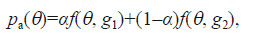
The spectral upwelling transmittances Tu (λ) were derived from the spectral downwelling plane transmittances Td, p(λ)(see definition of plane transmittance in Sokoletsky et al., 2014b) by applying the reciprocity principle (Sekera, 1970 ; Yang and Gordon, 1997). The upwelling radiance at the top of the atmosphere (TOA) level caused by the molecules (Rayleigh scattering) LR, TOA (λ) and aerosol particles La, TOA (λ) was modeled separately, in accordance with the Gordon and Castaño (1987) and Rahman and Dedieu (1994) assumptions. The two-term Henyey- Greenstein (TTHG) scattering phase function (Gordon and Castaño, 1987):
 (1)
(1)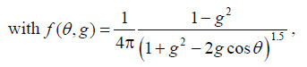 (2)
(2)where θ is a scattering angle and g is asymmetry parameter, has been used to present aerosol particles. The parameters α(λ), g1, and g2(λ) were set as functions of λ and τa (550) following the approximations suggested by Sturm and Zibordi (2002).
The spectral sun glitter radiance at the TOA level Lg, TOA (λ) has been estimated by the air-water statistical model developed by Cox and Munk (1954) and extended by Gordon and Voss (2004). A condition of the sun glitter avoidance has been implemented as described by Remer et al.(2005).
Finally, the Rrs (λ) values were derived from the TOA spectral upwelling radiance measured by the satellite sensor Lu, TOA (λ) by using equation:
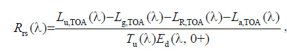 (3)
(3)where Ed (λ, 0+) is the modeled spectral global (from the sun and sky) atmospheric incident irradiance.
2.3 Deriving Rrs (λ) and ρ sky (λ) from radiometric measurementsThe first step in developing the retrieval SSC model is an analysis of in situ measurements, particularly, radiometric measurements. The spectral water-leaving radiance Lw (λ) may be expressed as
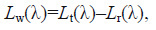 (4)
(4)where Lt and Lr are the total above-water radiance and the surface-reflected incident (sun+sky) radiance, respectively. Here we omit an impact of white caps on the Lt because this impact is generally insignificant compare to the total radiance; this is especially true for the case of turbid waters with a substantial inorganic content. Thus, a Lw (λ) can be estimated if an accurate estimate of Lr (λ) can be obtained.
Now we rewrite an Eq.4 in the form:
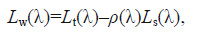 (5)
(5)where ρ(λ) is the spectral radiance reflectance that is affected by the geometrical conditions for sun and sensor, wavelength, wind speed, the sky radiance distribution, and field of view (Mobley, 1999 ; Lee et al., 2010). The ρ(λ) appears to be a highly variable parameter, especially as a function of the illumination conditions (Doxaran et al., 2004 ; Aas, 2010) and wavelength (Lee et al., 2010 ; Sokoletsky and Shen, 2014).
Below we consider six different models for deriving Rrs (λ)= Lw (λ)/ Ed (λ) from radiometric quantities.
2.3.1 Mobley model (MM)Mobley (1999) numerically calculated the ρ values for various geometrical and cloud conditions and wind speeds W. His results may be described by the following equation:
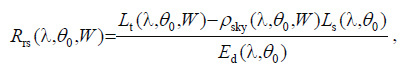 (6)
(6)where ρsky (λ) is the sky radiance spectral reflectance. The ρsky (λ) is assumed to be 0.028 for the heavily overcast sky at all values of λ, W and clear sky conditions at the wind speed W < 5 m/s, viewing zenith angle (VZA)θv =40°, azimuthal viewing direction of ϕv =135°, and SZA θ0 >10°(Fig. 9, Table 1 and S ection 7 in Mobley, 1999). In most cases of measurements at the YRE and its ACA these conditions were nearly satisfied; thus, we used a single value of ρsky =0.028 for this method. A selected observational geometry yields the sun glitter angle θg >47.5° that allows to neglect a sun glitter (ρ sun) for the MM and all other models (Remer et al., 2005).
In the earlier publications, like Whitlock et al.(1981), ρsky has been often accepted as 0.02 for any conditions. We used this value for estimation of Rrs (λ) by Eq.6 in the WM model.
2.3.3 Ruddick-Mobley model (RMM)This model based on Eq.6 with the ρsky calculated as a function of W and taking the ratio of Ls (750)/ Ed (750) into account according to Ruddick et al.(2006) :
 (7)
(7)For this model (Toole et al., 2000) the Fresnel's reflectance ρ Fr and two empirical (correction) parameters, c1 and c2 were introduced into Eq.6 as follows:
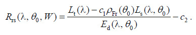 (8)
(8)The coefficients c1 and c2 are given in the Table 7 by Toole et al.(2000) for the wind speeds W ≤5 m/s and W >5 m/s, and for the clear, broken (foggy or cloudy), and diffuse (overcast) skies. The refractive index of the water for calculation of ρ Fr was accepted as 1.336.
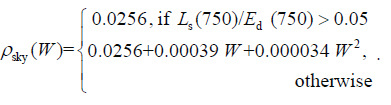
2.3.5 Simis-Olsson model (SOM)This model Rrs (λ) is estimated by Eq.6 with the ρsky calculated as in Sokoletsky and Shen (2014) :
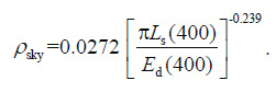 (9)
(9)This equation has been derived from 3 000 observations carried out by Simis and Olsson (2013) in the Baltic Sea.
2.3.6 Sokoletsky-Aas model (SAM)Here we assume that an optical instrument pointing to the sky measures not only sky (diffuse) light, but also sun (direct) light. Then, introducing a parameter dE (“irradiance diffuseness”) as the ratio of sky (diffuse) incident irradiance Ed, sky to the total (sky+sun) incident irradiance Ed (Woźniak, 1997), we get from Eqs.4 and 6
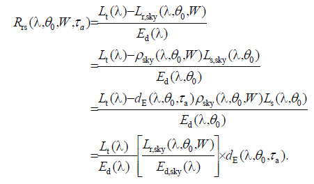 (10)
(10)Here we used the expression for ρsky (λ) as a ratio of the spectral reflected sky radiance just above the airwater surface Lr, sky (λ) to the spectral incident sky radiance Ls, sky (λ), and assuming that Ls, sky (λ)= dE (λ) Ls (λ). For this model, we expressed the spectral ratio Lr, sky (λθ0 W)/Ed, sky (λ) as follows (Aas, 2010 ; Sokoletsky and Shen, 2014):
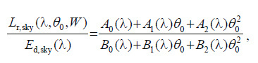 (11)
(11)where coefficients A0 - A2 and B0 - B2 are given in Aas (2010) as functions of wavelength λ(at 405, 450, 520, 550, and 650 nm) and wind speed W (at 0, 5, and 10 m/s) at solar zenith angles θ0 ranging from 37° to 76°. We performed calculations for any values of λ and W by linear interpolations and extrapolations, but taking θ0 =37°, if θ0 ≤37°, and θ0 =76°, if θ0 ≥76°.
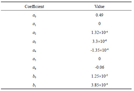
We have used the following analytical approximation for the spectral parameter dE (λ) derived from the atmospheric radiative transfer modeling (Sokoletsky et al., 2014a, c):
 (12)
(12)where θ0 in degrees, λ in nm, and all coefficients are given in the Table 1.
The spectral plots of ρsky (λ)(Fig. 4) and ρsky (λ) dE (λ)(Fig. 5) demonstrate a strong increasing of these parameters with λ for clear skies, the more temporal increasing for broken (cloudy or foggy) skies, and almost neutral behavior in the case of overcast skies. These facts differentiate the SAM model from the others, for which no dependency of ρsky versus λ is assumed. Note also an agreement of this conclusion with findings of Lee et al.(2010) and Sokoletsky and Shen (2014).

|
| Figure 4 The mean (±standard deviations) values of the spectral sky radiance reflectance ρsky (λ) computed for the 54 samples collected during February 17 to March 10, 2014 in the East China coastal area by the SAM model with the sky conditions taken into account |

|
| Figure 5 The same as Fig. 3, but for the ρsky (λ) dE (λ) |
It is remarkable that models MM, WM, RMM, and SOM have a similar design as Eq.6. The difference between these four models is caused only by different expressions for the sky radiance spectral reflectance ρsky (λ). However, the TM model adds two empirical coefficients to better take into account the wind and sky conditions. The SAM model is similar on its structure to the TM model, if to assume that the parameter c1(from the TM model) is similar to the parameter dE (from the SAM model) and c2 =0. However, the dE is much more sensitive to the diffuseness of incident light than the c1 in the TM model. Mathematical analysis of Eqs.6, 8, and 10 shows that an Eq.10(i.e., the SAM model) could yield bigger values for Rrs (λ) than Eqs.6 and 8.
This mathematical analysis is confirmed by numerical calculations showing generally the biggest spectral values of Rrs (λ) for the SAM model and the smallest values for the TM model. Moreover, the TM model sometimes shows negative values in visible, ultraviolet, and NIR spectral ranges, while the other models show either only positive values (WM) or negative values only in the NIR spectral range (MM, RMM, SOM, and SAM). For the whole spectral range of 350-900 nm, negative Rrs (λ) values were obtained in 0%, 0.7, 1.1%, 2.6%, 3.1%, and 25% cases for WM, RMM, SAM, SOM, MM, and TM models, respectively. We explain the significantly large percentage of negative Rrs (λ) values in the case of TM model by the large difference between environmental conditions in which the TM model was parameterized and conditions in which our measurements were performed. For example, the SSC values varied from 0.0 to 3.4 g/m3 and from 3.9 to 475 g/m3 in Toole et al.(2000) site of interest (the Santa Barbara Channel) and in our geographical area, respectively. Therefore, the SAM model based on the strong radiative transfer considerations and which yields generally positive Rrs (λ) values was selected as the main model for the further modeling.
Below we compare the six models described above for the Rrs (λ) retrieval for only two observation dates under clear (Fig. 6a) and cloudy (Fig. 6b) sky conditions. The differences between the SAM and all other models are generally smaller in clear sky conditions. To estimate numerically an impact of sky conditions on the differences between five models (the TM model has been excluded here from consideration), all samples were divided by three groups, namely, collected during clear (21 samples), cloudy or foggy (20 samples), and overcast (13 samples) skies. The results were expressed via the spectral variation coefficient Var (λ) for Rrs (λ)(Fig. 7) equal to the standard deviation of the Rrs (λ) normalized by the mean Rrs (λ) value calculated for each wavelength. Results confirm an increase in models' deviations with increasing atmospheric diffuseness. Notice also a general increasing of Var (λ) in the NIR comparative to the visible spectral range.

|
| Figure 6 The comparison between the Rrs spectra derived by different models from radiometric in situ measurements performed during (a) March 9, 2014, UTC06:18 under clear sky conditions on the station with coordinates: 122.248 9°E, 30.640 1°N and (b) February 20, 2014, UTC03:23 under cloudy sky conditions on the station with coordinates: 121.797 7°E, 31.233 6°N |

|
| Figure 7 The mean (±standard deviations) values of the Rrs (λ) variation coefficient computed for the 54 samples collected during February17 to March 10, 2014, in the East China coastal area for five models (the TM model has been excluded from consideration) with the sky conditions taken into account |
All symbols referred to the samples collected during February 17 to March 10, 2014, in the East China coastal area. Note that this figure is a type of a scatter plot with the omitted x-axis labels. This type has been chosen intentionally to stress a missing relationship between the values of two coordinates.
Even though numerical differences between Rrs (λ) estimated by different models may be large enough, using spectral ratios significantly decreases such differences (Sokoletsky and Gallegos, 2010 ; Wang et al., 2010b). Below (Fig. 8) we test six abovementioned models for the spectral ratio of Rrs (645.5)/ Rrs (553.6) at different sky conditions. The 645.5 and 553.6 nm are the central wavelengths of the first and fourth MODIS bands, respectively (Neteler, 2014), and their ratio was found to be usable for the remote sensing of water quality parameters in the YRE and ACA (Sokoletsky et al., 2014a). The Fig. 8 clearly shows that using the spectral ratio decreases the difference between the models, but this difference depends strongly on the spectral ratio value. More specifically, the models generally underestimate SAM values when this ratio approximately<1, and overestimate SAM values at Rrs (645.5)/ Rrs (553.6)>1, independently of sky conditions. Overall, the maximal discrepancies were found between the TM and all other models. Excluding again the TM model from consideration, we obtained the mean variation coefficient between the five models of 4.6(±7.5)%, 11(±15)%, and 16(±12)% for clear, broken (cloudy or foggy), and overcast sky conditions, respectively. Thus, accounting that remote sensing imagery is performed effectively under clear skies, using the Rrs (645.5)/ Rrs (553.6) seems to be safe enough for exploring in the YRE and its ACA area of China.

|
| Figure 8 A plot illustrating the Rrs (645.5)/ Rrs (553.6) spectral ratio computed by different radiometric models (shown in the legend) and under different sky conditions: clear (a), broken (b), and overcast (c) skies |
The Rrs (λ) versus SSC relationships follow from 1) relationships between the IOPs (spectral absorption a (λ), scattering b (λ), and backscattering bb (λ) coefficients) and SSC; 2) relationships between the spectral subsurface remote-sensing reflectance rrs (λ), IOPs and measurement geometry conditions; and 3) relationships between the rrs (λ) and Rrs (λ). Below we consider these issues in some more details.
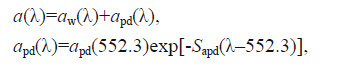
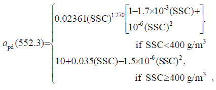
2.4.2 Relationships between the IOPs and SSCA mathematical modeling has shown that the a (λ) dependency characterized by the spectrally non-flat curve with a shift of the spectral absorption minimum from the blue to NIR at increasing SSC (Fig. 9a) while the both b (λ)(Fig. 9b) and bb (λ)(Fig. 9c) dependencies are spectrally flat with the strong decrease toward the NIR spectral range at any SSC. Mathematically, these dependencies may be described as follows:
 (13)
(13) (14)
(14) (15)
(15) (16)
(16) (17)
(17) (18)
(18) (19)
(19) (20)
(20)

|
| Figure 9 The spectral optical model relating a (λ)(a), b (λ)(b), bb (λ)(c), and G (λ)(d) with SSC for the study area |
where all optical properties are expressed in inverse meters, SSC in g/m3, and λ in nm; the subscripts w, p, and d refer to water, particles, and dissolved matter, respectively. The aw (λ) values were interpolated from the Table V-1 by Lu (2006) at λ<600 nm, from Table 3 by Pope and Fry (1997) at 600≤λ<736 nm, from Table 1 by Buiteveld et al.(1994) at 736≤λ<801 nm, and from the webpage by Prahl and Jacques (1998) [based on the refractive indices by Kou et al.(1993) ] at λ≥801 nm. An expression for the bw (λ) has been derived from the optical model by Zhang et al.(2009) at the temperature of 20℃ and salinity of 30 g/kg, λ=300 to 1 000 nm (with the mean absolute percentage error of 1.4% and R2 of 0.998 2). The bbw (λ) has been assumed to be exactly a half of the bw (λ).
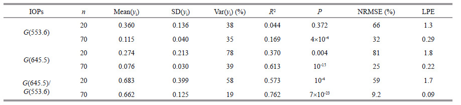
The Eqs.13-20 have been used for estimation of the spectral Gordon's parameter G (λ)= bb (λ)/ [ a (λ)+ bb (λ)](Fig. 9d), which may be considered as a spectral proxy for the Rrs (λ) in the first approximation (Haltrin and Gallegos, 2003 ; Sokoletsky et al., 2012 ; Sokoletsky and Fang, 2014).
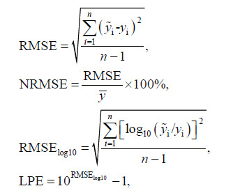
We calculated this parameter (Table 2) at two MODIS wavelengths: 553.6 and 645.5 nm as a function of measured SSC for the May 2011 and February-March 2014 datasets. The accuracy of the model for G (553.6), G (645.5), and G (645.5)/ G (553.6) has been determined by the following statistical measures: determination coefficient R2, normalized root-mean-square error NRMSE, and the linear percentage error LPE. The two last measures were calculated as follows (Lee et al., 2002 ; Sokoletsky et al., 2012):
 (21)
(21)
|
where y i and ${\tilde{y}}$i are observed and predicted IOPs for the i th sample, respectively; n is the sample size; y is the observed mean value; and RMSElog10 is the rootmean- square error in log 10 scale. Table 2 contains these results along with the standard deviation, SD (yi) and variability, Var (yi)=[SD (yi)/ y]×100% for G (553.6), G (645.5), and G (645.5)/ G (553.6).The table shows that using the spectral ratio G (645.5)/ G (553.6)[and, hence, the Rrs (645.5)/ Rrs (553.6)] is generally more numerically accurate than using the single wavelengths G (λ) values. A similar conclusion can be drawn for the correlation between predicted and measured G (λ).
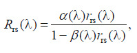
2.4.3 Relationships between the rrs (λ), IOPs and measurement geometry conditionsThe subsurface remote-sensing reflectance rrs (λ)= Lu (λ, 0-)/ Ed (λ, 0-) may be estimated from IOPs and measurement geometry conditions, for instance, by any of the five accurate approximations suggested and tested in Gordon et al.(1988), Lee et al.(1999), Albert and Gege (2006), Sokoletsky et al.(2009, 2012), and Sokoletsky and Shen (2014). We have used the combined Sokoletsky et al.(2012) and Albert and Gege (2006) approximation for rrs (λ)(Albert and Gege, 2006 ; Sokoletsky et al., 2012 ; Sokoletsky and Shen, 2014):
 (22)
(22)where μ1 and μ2 are cosines of SZA and VZA, respectively, just below the air-sea surface.
2.4.4 Relationships between the rrs (λ) and Rrs (λ)The model Rrs (λ) values were derived from the rrs (λ) by the following approximation:
 (23)
(23)where α(λ)= 0.3638 + 8.776 × 10⁻⁴ λ - 9.193 × 10 - 7 λ 2 + 3.174 × 10 - 10 λ 3 and β(λ)=1.357+8.608 × 10⁻⁴ λ-6.347 × 10 - 7 λ 2(λ in nm). Equation 23 has been derived from the radiative transfer Aas-Højerslev model (Højerslev, 2001 ; Aas, 2010 ; Sokoletsky and Shen, 2014) at the solar zenith angle θ0 =40°, W =5 m/s, and wavelengths of 400-800 nm with R2 =0.999 5 and R2 =0.990 3 for α(λ) and β(λ), respectively.
2.4.5 Relationships between the Rrs (λ) and SSCFigure 10 shows the model dependencies of Rrs (λ, SSC) at θ0 =θ v= 40° and wide ranges of λ and SSC computed by three steps in the manner described above, namely: 1) SSC→IOPs (Subsection 2.4.2); 2) IOPs→ rrs (λ)(Subsection 2.4.3); and 3) rrs (λ)→ Rrs (λ)(Subsection 2.4.4).

|
| Figure 10 The spectral optical model relating Rrs with SSC (shown in the legend of (a) in g/m3 units) and wavelength (shown in the legend of (b) in nm units) derived from the YRE and its ACA data The solar zenith θ0 and viewing zenith θv angles assumed as 40° |

|
| Figure 11 The relative errors in R r s (λ=550 nm, θ0, θv) vs. Rrs (λ=550 nm, θ0 =40°, θv =40°) A blue rectangle illustrates an area for errors caused by SZA variations during the February 17 to March 10, 2014 data collection, while the green rectangle indicates an area for errors caused by possible errors in VZA. |
An important feature of the Rrs (λ, SSC) spectral behavior is an almost exact coincidence of a (λ, SSC) spectral minima (Fig. 9a) with the Rrs (λ, SSC) spectral maxima (Fig. 10a). Another important feature is an almost linear character of Rrs (λ) vs. SSC at small SSC (Fig. 10b). However, a relationship between SSC and Rrs (λ) becomes flatter with the SSC increasing. Fig. 10b demonstrates a shift of the SSC boundary between linear and nonlinear relationships with the increasing wavelength. For example, at wavelengths of 412-532, 595-676, 715, and 865 nm the boundary is achieved at SSC about 6, 10, 20, and 600 g/m3, respectively. These findings are in a qualitative accordance with the previous studies (Harrington Jr et al., 1992 ; Han and Rundquist, 1994 ; Wang and Lu, 2010 ; Shen et al., 2010a ; Qu, 2014).
One can use the angles θ0 and θv different from 40°, which may lead to small differences from the results shown in Fig. 10. An analysis of errors in Rrs (λ θ0, θv) at λ=550 nm caused by different θ0 and θv is given in Annex. The relative errors in Rrs (λ=550 nm, θ0, θv) vs. Rrs (λ=550 nm, θ0 =40°, θv =40°) derived from Eqs.A1 and A3 are shown in Fig. 11. Numerically, they do not exceed 5% for the observational conditions during data collection.
2.4.6 Comparison between different Rrs (λ) versus SSC relationshipsA large variability of different combinations of spectral reflectance may be used for SSC retrievals (Ma and Dai, 2005 ; Zhou et al., 2006 ; Ouillon et al., 2008), that makes the choice of the spectral SSC model a non-trivial task. Such models are inherently different for specific geographical sites and seasons, and even for different hours of the day.
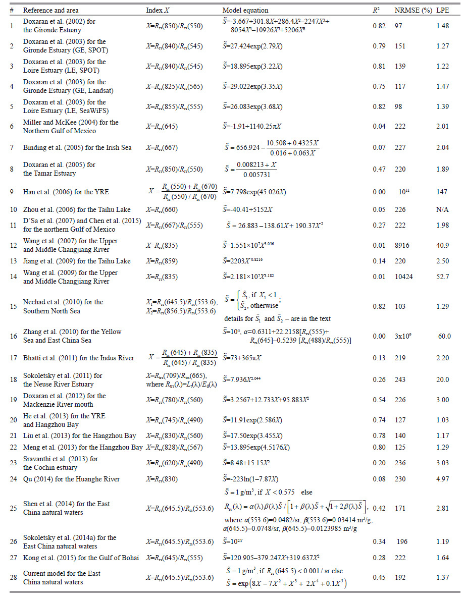
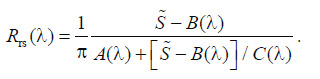
Below (Table 3) we compare numerous SSC retrieval models developed for the turbid Case 2 waters based on different indices X. Testing these models was realized for the laboratory tank and in situ data (see Section 2.1) with the wavelengths taken from either the middle of the spectral ranges, or from the central wavelengths indicated by the authors. The basic Rrs (λ) values were derived from radiometric measurements, θ0, τ a (λ) and W by the SAM method (Subsection 2.3.6). Table 3 lists literature models with the corresponding values of R2, NRMSE, and LPE, calculated similarly to those measures applied to the IOPs (Eq.21). In case of necessity for modeling, the spectral water-leaving reflectance ρw (λ) has been replaced by Rrs (λ) according to the simple equation: ρw (λ)=π Rrs (λ)(Jerlov, 1976, p. 79; Gordon and Voss, 2004 ; Ruddick et al., 2006 ; Sokoletsky and Shen, 2014).
|
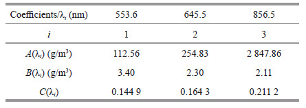
The Nechad et al.(2010) model was exploited as a function of the spectral ratios formed for three central MODIS wavelengths: λ1 =553.6, λ2 =645.5, and λ3 =856.5 nm. This model has been derived from the generic spectral equation (Nechad et al., 2010):
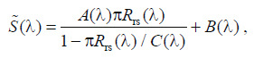 (24)
(24)where spectral coefficients A (λ), B (λ), and C (λ) were interpolated from Nechad et al.(2010) as follows (Table 4):
Below we present a derivation of the spectral ratios version of this algorithm. It is follows from Eq.24:
 (25)
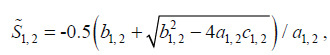
(25)Two quadratic equations may be formulated, if to write an Eq.24 for all three wavelengths and to form two ratios, namely, X1 = Rrs (λ2)/ Rrs (λ1) and X2 = Rrs (λ3)/ Rrs (λ1), as functions of $\tilde{S}$. Two different solutions of these equations for $\tilde{S}$($\tilde{S}$ 1 and $\tilde{S}$ 2) are as follows:
 (26)
(26)where
 (27)
(27)with the coefficients A i, B i, and C i meaning A (λi), B (λi), and C (λi), where i =1, 2, 3 from the Table 4.
A similar approach was applied to the semiempirical model by Shen et al.(2014). This model initially developed for individual wavelengths was adjusted for the Rrs (645.5)/ Rrs (553.6) spectral ratio (Table 3). A pair of coefficients (α and β) necessary for this model at wavelengths of 553.6 and 645.5 nm was derived by linear interpolation of values used in Table 2 by Shen et al.(2014). As noted in Shen et al.(2014), a spectral reflectance ratio approach leads to underestimated or even negative values SSC for relatively clear waters. To avoid this situation, a condition: SSC=1 g/m3, if Rrs (645.5)/ Rrs (553.6)<0.575 has been added to the model.
The currently used model (#28) has been developed as a modification of the earlier derived MODIS model (Sokoletsky et al., 2014a). The new model is derived from the measured SSC and Rrs (λ) values and it numerically close to the model values derived from the IOPs vs. SSC equations (Eqs.13-20), Eq.22 for rrs (λ) vs. IOPs, and Eq.23 for Rrs (λ) vs. rrs (λ).
Overall, of the 28 models listed in Table 3, the seven models use the single wavelength (in the red or NIR ranges) for the SSC retrieval while the simple spectral ratios were used in the 17 models. Han et al.(2006), Nechad et al.(2010), Zhang et al.(2010), and Bhatti et al.(2011) used some more complicated functions of the spectral reflectance. The models by Doxaran et al.(2002), Nechad et al.(2010), He et al.(2013), Liu et al.(2013), Meng et al.(2013), Shen et al.(2014), Sokoletsky et al.(2014a), and currently used MODIS model (#28) have been demonstrated to provide the best results (from statistics and visual perception points of view)(Fig. 12).

|
| Figure 12 Examples of the SSC model results plotted versus measured SSC values a. Doxaran et al.(2002) ; b. Nechad et al.(2010) ; c. He et al.(2013) ; d. Liu et al.(2013) ; e. Meng et al.(2013) ; f. Shen et al.(2014) ; g. Sokoletsky et al.(2014a) ; h. the current MODIS-AA model (#28). AA means here an analytical algorithm. |
Interestingly to note that among these eight models, the He et al.(2013), Liu et al.(2013), Meng et al.(2013), Shen et al.(2014), Sokoletsky et al.(2014a), and the current MODIS-AA (#28) models have been derived from the East China natural waters (YRE with its ACA, Yellow Sea, Taihu Lake and Hangzhou Bay), while the Doxaran et al.(2002) and Nechad et al.(2010) models were obtained for the Gironde Estuary and the Southern North Sea, respectively. Overall, the currently developed MODIS-AA model (#28) seems to be the superior model. However, a total accuracy and correlation with the measured SSC values for all models, even for the best ones, is still relatively poor (Table 3); this may be explained mainly by: 1) a mismatch between literature study geographical areas and our areas; 2) a large variability of IOPs vs. SSC relationships (Table 2); and 3) inaccuracies of measurements and models themselves.
2.4.7 The SSC versus spectral Rrs (λ) ratio relationshipFigure 13 confirms the reability of using the red-togreen models by Nechad et al.(2010), Shen et al.(2014), Sokoletsky et al.(2014a), and the current MODIS-AA model (#28) for SSC retrieval in the East China natural waters. The figure also confirms that these four SSC models are robust yielding appropriate results for the datasets collected in different times in the East China coastal area.

|
| Figure 13 The SSC versus the X = Rrs (645.5)/ Rrs (553.6) spectral ratio for tank and two field datasets The determination coefficients of exponential relationships between the spectral ratio and SSC for each dataset shown in rectangulars colored by the same color as datasets ’ points. The solid, dashed, dash-dotted, and dotted black lines correspond to the model equations by Nechad et al.(2010) (at X <1), Shen et al.(2014), Sokoletsky et al.(2014a), and the current MODIS-AA model (#28). |
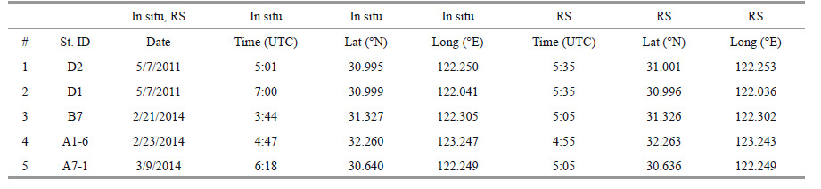
Each match-up Rrs (λ) curve has the same color as the associated in situ Rrs (λ) curve, and is numbered following Table 5.
|
A larger part of AC algorithm has been already confirmed by previous investigations. For example, a REST2 solar irradiance model by Gueymard (2008), many elements of which are used in the present study, has been validated by help of benchmark dataset. The two stream radiative transfer model used in our AC algorithm for transmittances by atmospheric molecules and aerosols has been successfully validated by comparison with numerical results derived from the Herman and Browning (1965) radiative transfer solution. Finally, transmittance of upwelling radiance was modeled following the reciprocity principle theoretically derived and validated by Sekera (1970) and Yang and Gordon (1997).
A comparison of the field-based reflectance spectra with the MODIS-derived Rrs (λ) spectra and SSC is another way to validate our AC and SSC algorithms. Unfortunately, only five in situ-remote sensing couples with the relatively small space (<700 m) and temporal (<1.4 hours) differences could be used for validation (Table 5, Fig. 14). The Rrs (λ) spectra of the field and satellite datasets demonstrate close numerical values, spectral form, and the peak position. The closeness of the spectral forms for in situ and remote sensing data stimulates using the Rrs (λ) ratios (Fig. 15) for remote sensing water quality monitoring in the study area.

|
| Figure 14 The in situ Rrs (λ)(solid curves) and their associated match-up Rrs (λ)(dashed curves with symbols) spectra |

|
| Figure 15 The scattering plot of in situ-measured and the MODIS-derived Rrs (645.5)/ Rrs (553.6) spectral ratios (a) and SSC (b) for the same locations and times as shown in Table 5 AA means here an analytical algorithm. |
Figure 16 shows examples of the color (false) images for the SSC in the East China coastal area, 2008 -2013. All images were produced based on the AC and SSC estimation algorithms described above and have shown reasonable values, comparable with the literature data. For example, SSC in the ECS area were found relatively small: ~1 to 70 g/m3that is close to the values found by Kiyomoto et al.(2001), Shen et al.(2010a, 2013, 2014), Siswanto et al.(2011), and He et al.(2012, 2013). The SSC concentration values in the Taihu Lake lie in the range of ~19-150 g/m3that corresponds to the values reported by Zhou et al.(2006), Jiang et al.(2009), Hu et al.(2010), He et al.(2012, 2013), Zhao et al.(2013), and Shen et al.(2014).

|
| Figure 16 The SSC retrieved images of the East China natural waters acquired on different dates during 2008-2013 AA means here an analytical algorithm. |
Figure 16 demonstrates the extremely high SSC values achieved in the YRE (~20-750 g/m3), Hangzhou Bay (~70-3 300 g/m3), and the Subei Bank of the Yellow Sea (~80-2 500 g/m3) that also confirmed by numerous studies, e.g., Li et al.(1994), He et al.(1999), Han et al.(2006), Salama and Shen (2010), Shen et al.(2010a, b, 2013, 2014), Shi and Wang (2010), Wang et al.(2010a), Zhang et al.(2010), He et al.(2012, 2013), Li et al.(2012), and Liu et al.(2013). Note that we rejected here some SSC values appeared too high (totally ~2% of all values), which may be caused by wrong pixel identification (e.g., in case of thin clouds, hardly identified by the AC algorithm).
4 CONCLUSIONThe study revealed several important points concerning in situ observations and satellite remotesensing of water quality in the East China natural waters:
1. The area is characterized by the extremely wide range of SSC variations: from ~1 to 3 300 g/m3(Figs. 2, 3, 16). The SSC concentration values are closely related to the quality of water (Figs. 2, 3); however, such correlation was not found for Chl concentration. Also, no significant correlation was found between SSC and Chl. Thus, our study shows that the SSC cconstitutes the main impact on water quality in the area. Therefore, the water quality components estimation methods based on the close relationships between Chl and SSC (like methods described by Sokoletsky et al., 2011, 2012) are probably inadequate in the East China area;
2. Measurements and modeling results demonstrated a strong spectral dependency for the diffuse light reflectance ρsky (λ) and ρsky (λ) dE (λ) during clear sky hours; however, such dependency is weakened with the degree of cloudiness (Figs. 4, 5). This fact allows using more elaborated radiative transfer air-water modeling (like has been described in Subsection 2.3.6) for in situ above-water measurements with the aim of better support of remote-sensing observations;
3. A comparison between different radiometric Rrs (λ) models have shown a relatively small variability (below 20% for five best models) between the models in the case of clear sky conditions in the whole 400- 900 nm spectral range (Figs. 6, 7). However, variability increases with increasing atmospheric cloudiness or diffuseness, especially in the NIR range (up to 100% and more). Thus, this modeling shows that the fieldbased estimation of Rrs (λ), like the remote-sensing estimation of this parameter, is more reliable if the radiometric data are collected during clear sky conditions.
A further decrease in discrepancies between different Rrs (λ) models has been found using the spectral Rrs (λ) ratios (Fig. 8 provides an example). In any case, the SAM model appeared as a more elaborated radiative transfer model, yielding only 1.1% negative values in the whole 350-900 nm spectral range;
4. Figures 9 and 10 demonstrate important feature of the Rrs (λ, SSC) relationships, namely, an almost exact coincidence of Rrs (λ, SSC) spectral maxima with the a (λ, SSC) spectral minima. This fact may be useful for understanding the spectral features of Rrs (λ) and for remote-sensing retrieval of IOPs. Another important feature of the Rrs (λ, SSC) relationships is an almost linear increasing with SSC at relatively small SSC; then, with increasing SSC, dependency becomes slower, and finally almost invariable with SSC (Fig. 10). This fact explains the success of different (linear and nonlinear) models for different water situations. For example, at wavelengths of 412-532, 595-676, 715, and 865 nm, a linear part of Rrs vs. SSC relationship lasts up to 6, 10, 20, and 600 g/m3, respectively (Fig. 10b), that allows to develop the linear, but still accurate algorithms for relatively clear waters. However, for a general case of widely varied SSC more complicated methods are needed;
5. The model computations have shown (Table 2) a preference of using the method of the spectral ratios (relative to the single wavelengths approach) in terms of accuracy and correlation between predicted and measured optical properties;
6. An analysis of errors caused by possible variations in the solar and viewing zenith angles has shown their small impact (within 5%-10%) on the spectral reflectance dependency on IOPs (Fig. 11). Moreover, using spectral Rrs (λ) ratios cancels an angular impact almost completely. This confirms the similar conclusions obtained before from the more elaborated numerical analysis (Sokoletsky and Gallegos, 2010);
7. The comparison study of 28 different SSC vs. Rrs (λ)[or ρw (λ) or R trs (λ)] models taken from literature have revealed several models (based on investigations in Chinese and non-Chinese natural waters) yielding robust results relatively close to our observational data (Fig. 12);
8. The study confirmed the reliability of using the red-to-green models for SSC retrieval (Fig. 13);
9. A new empirical SSC vs. Rrs (645.5)/ Rrs (553.6) model along with the atmospheric correction based on the analytic radiative transfer algorithm (Sokoletsky et al., 2014a) were applied for SSC mapping of inland, estuarine and coastal waters of the East China (Fig. 16). An analysis of these maps has shown their common compatibility with the published data. A validation of the atmospheric correction algorithm has been provided by comparison with the in situ measured reflectance spectra and spectral Rrs (645.5)/ Rrs (553.6) ratio (Figs. 14, 15).
Thus, it is feasible, given the rigorous nature of our approach, to consider the further application of developed AC-SSC algorithm not only for the area under study, but also for the other areas around the world.
5 ACKNOWLEDGEMENTWe thank Dr. Chris Gueymard from the Solar Consulting Services for the valuable discussion on the optical atmospheric model. We would like also to express our gratitude to the two anonymous reviewers for their extremely constructive and helpful feedback on earlier drafts of this paper.
| Aas E, 2010. Estimates of radiance reflected towards the zenith at the surface of the sea. Ocean Sci., 6 (4) : 861 –876. Doi: 10.5194/os-6-861-2010 |
| Albert A, Gege P, 2006. Inversion of irradiance and remote sensing reflectance in shallow water between 400 and 800 nm for calculations of water and bottom properties. Appl. Opt., 45 (10) : 2331 –2343. Doi: 10.1364/AO.45.002331 |
| Ben-David A, 1995. Multiple-scattering transmission and an effective average photon path length of a plane-parallel beam in a homogeneous medium. Appl. Opt., 34 (15) : 2802 –2810. Doi: 10.1364/AO.34.002802 |
| Ben-David A, 1997. Multiple-scattering effects on differential absorption for the transmission of a plane-parallel beam in a homogeneous medium. Appl. Opt., 36 (6) : 1386 –1398. Doi: 10.1364/AO.36.001386 |
| Binding C E, Bowers D G, Mitchelson-Jacob E G, 2005. Estimating suspended sediment concentrations from ocean colour measurements in moderately turbid waters; the impact of variable particle scattering properties. Remote Sens. Environ., 94 (3) : 373 –383. Doi: 10.1016/j.rse.2004.11.002 |
| Buiteveld H, Hakvoort J H M, Donze M, 1994. Optical properties of pure water. In: Jaffe J S ed. Proceedings of SPIE, Ocean Optics XⅡ. SPIE, Bergen, Norway, 2258 : 174 –183. |
| Chen J, Quan W T, Cui T W, Song Q J, 2015. Estimation of total suspended matter concentration from MODIS data using a neural network model in the China eastern coastal zone. Estuarine, Coastal and Shelf Science, 155 : 104 –113. Doi: 10.1016/j.ecss.2015.01.018 |
| Cox C, Munk W, 1954. Measurement of the roughness of the sea surface from photographs of the sun's glitter. J. Opt.Soc. Am., 44 (11) : 838 –850. Doi: 10.1364/JOSA.44.000838 |
| Cracknell A P, 1999. Twenty years of publication of the International Journal of Remote Sensing. Int. J. Remote Sens., 20 (18) : 3469 –3484. Doi: 10.1080/014311699211138 |
| D'Sa E J, Miller R L, McKee B A, 2007. Suspended particulate matter dynamics in coastal waters from ocean color:application to the northern Gulf of Mexico. Geophys. Res.Lett., 34 (23) : L23611 . Doi: 10.1029/2007GL031192 |
| Doxaran D, Cherukuru R C N, Lavender S J, 2004. Estimation of surface reflection effects on upwelling radiance field measurements in turbid waters. J. Opt. A: Pure Appl. Opt., 6 (7) : 690 –697. Doi: 10.1088/1464-4258/6/7/006 |
| Doxaran D, Cherukuru R C N, Lavender S J, 2005. Use of reflectance band ratios to estimate suspended and dissolved matter concentrations in estuarine waters. Int. J.Remote Sens., 26 (8) : 1763 –1769. Doi: 10.1080/01431160512331314092 |
| Doxaran D, Ehn J, Bélanger S, Matsuoka A, Hooker S, Babin M, 2012. Optical characterisation of suspended particles in the Mackenzie River plume (Canadian Arctic Ocean)and implications for ocean colour remote sensing. Biogeosciences, 9 (8) : 3213 –3229. Doi: 10.5194/bg-9-3213-2012 |
| Doxaran D, Froidefond J M, Castaing P, 2002. A reflectance band ratio used to estimate suspended matter concentrations in sediment-dominated coastal waters. Int.J. Remote Sens., 23 (23) : 5079 –5085. Doi: 10.1080/0143116021000009912 |
| Doxaran D, Froidefond J M, Castaing P, 2003. Remote-sensing reflectance of turbid sediment-dominated waters. Reduction of sediment type variations and changing illumination conditions effects by use of reflectance ratios.Appl. Opt., 42 (15) : 2623 –2634. |
| Gordon H R, Brown O B, Evans R H, Brown J W, Smith R C, Baker K S, Clark D K, 1988. A semianalytic radiance model of ocean color. J. Geophys. Res., 93 (D9) : 10909 –10924. Doi: 10.1029/JD093iD09p10909 |
| Gordon H R, Castaño D J, 1987. Coastal Zone Color Scanner atmospheric correction algorithm: multiple scattering effects. Appl. Opt., 26 (11) : 2111 –2122. Doi: 10.1364/AO.26.002111 |
| Gordon H R, McCluney W R, 1975. Estimation of the depth of sunlight penetration in the sea for remote sensing. Appl.Opt., 14 (2) : 413 –416. Doi: 10.1364/AO.14.000413 |
| Gordon H R, Voss K J. 2004. MODIS normalized waterleaving radiance, algorithm theoretical basis document(MODIS 18), Version 5. University Miami, Coral Gables, FL, US. |
| Gueymard C A, 2001. Parameterized transmittance model for direct beam and circumsolar spectral irradiance. Solar Energy, 71 (5) : 325 –346. Doi: 10.1016/S0038-092X(01)00054-8 |
| Gueymard C A, 2003. Direct solar transmittance and irradiance predictions with broadband models. Part I: detailed theoretical performance assessment. Solar Energy, 74 (5) : 355 –379. |
| Gueymard C A, 2008. REST2: high-performance solar radiation model for cloudless-sky irradiance, illuminance, and photosynthetically active radiation-Validation with a benchmark dataset. Solar Energy, 82 (3) : 272 –285. Doi: 10.1016/j.solener.2007.04.008 |
| Gueymard C. 1995. SMARTS2: a simple model of the atmospheric radiative transfer of sunshine: algorithms and performance assessment. Report FSEC-PF-270-95, Florida Solar Energy Center, Cocoa, FL. |
| Haltrin V I, Gallegos S C. 2003. About nonlinear dependence of remote sensing and diffuse reflectance coefficients of Gordon's parameter. In: Levin I, Gilbert G eds. Proceedings of the Ⅱ International Conference "Current Problems in Optics of Natural Waters" ONW-2003. SaintPetersburg, Russia. p.363-369. |
| Han L, Rundquist D C, 1994. The response of both surface reflectance and the underwater light field to various levels of suspended sediments: preliminary results. Photogr.Eng. Remote Sens., 60 (12) : 1463 –1471. |
| Han Z, Jin Y Q, Yin C X, 2006. Suspended sediment concentrations in the Yangtze River estuary retrieved from the CMODIS data. Int. J. Remote Sens., 27 (19) : 4329 –4336. Doi: 10.1080/01431160600658164 |
| Harrington Jr J A, Schiebe F R, Nix J F, 1992. Remote sensing of Lake Chicot, Arkansas: monitoring suspended sediments, turbidity, and Secchi depth with Landsat MSS data. Remote Sens. Environ., 39 (1) : 15 –27. Doi: 10.1016/0034-4257(92)90137-9 |
| He Q, Yun C X, Shi F R, 1999. Remote sensing analysis of suspended sediment concentration in water surface layer in the Changjiang estuary. Progr. Nat. Sci., 9 (6) : 160 –164. |
| He X Q, Bai Y, Pan D L, Huang N L, Dong X, Chen J S, Chen C T A, Cui Q F, 2013. Using geostationary satellite ocean color data to map the diurnal dynamics of suspended particulate matter in coastal waters. Remote Sens.Environ., 133 : 225 –239. Doi: 10.1016/j.rse.2013.01.023 |
| He X Q, Bai Y, Pan D L, Tang J W, Wang D F, 2012. Atmospheric correction of satellite ocean color imagery using the ultraviolet wavelength for highly turbid waters. Optics Express, 20 (18) : 20754 –20770. Doi: 10.1364/OE.20.020754 |
| Herman B M, Browning S R, 1965. A numerical solution to the equation of radiative transfer. J. Atmos. Sci., 22 (5) : 559 –566. Doi: 10.1175/1520-0469(1965)022<0559:ANSTTE>2.0.CO;2 |
| Højerslev N K, 2001. Analytic remote-sensing optical algorithms requiring simple and practical field parameter inputs. Appl. Opt., 40 (27) : 4870 –4874. Doi: 10.1364/AO.40.004870 |
| Hu C M, Lee Z P, Ma R H, Yu K, Li DQ, Shang S L, 2010. Moderate resolution imaging spectroradiometer (MODIS)observations of cyanobacteria blooms in Taihu Lake, China. J. Geophys. Res., 115 (C4) . Doi: 10.1029/2009JC005511 |
| Jerlov N G, 1976. Marine Optics. Elsevier Scientific, New York : 230p . |
| Jiang X W, Tang J W, Zhang M W, Ma R H, Ding J, 2009. Application of MODIS data in monitoring suspended sediment of Taihu Lake, China. Chin. J. Oceanol. Limnol., 27 (3) : 614 –620. Doi: 10.1007/s00343-009-9160-9 |
| Kiyomoto Y, Iseki K, Okamura K, 2001. Ocean color satellite imagery and shipboard measurements of chlorophyll a and suspended particulate matter distribution in the East China Sea. J. Oceanogr., 57 (1) : 37 –45. Doi: 10.1023/A:1011170619482 |
| Kou L, Labrie D, Chylek P, 1993. Refractive indices of water and ice in the 0. 65- to 2.5-μm spectral range. Appl. Opt., 32 (19) : 3531 –3540. |
| Lee Z P, Ahn Y H, Mobley C, Arnone R, 2010. Removal of surface-reflected light for the measurement of remotesensing reflectance from an above-surface platform. Optics Express, 18 (25) : 26313 –26324. Doi: 10.1364/OE.18.026313 |
| Lee Z P, Carder K L, Arnone R A, 2002. Deriving inherent optical properties from the water color: a multiband quasianalytical algorithm for optically deep waters. Appl. Opt., 41 (27) : 5755 –5772. Doi: 10.1364/AO.41.005755 |
| Lee Z P, Carder K L, Mobley C D, Steward R G, Patch J S, 1999. Hyperspectral remote sensing for shallow waters: 2. deriving bottom depths and water properties by optimization. Appl. Opt., 38 (18) : 3831 –3843. |
| Li D J, Dag D, 2004. Ocean pollution from land-based sources:East China Sea, China. AMBIO, 33 (1) : 107 –113. Doi: 10.1579/0044-7447-33.1.107 |
| Li J F, Shi W R, Shen H T, 1994. Sediment properties and transportation in the turbidity maximum in Changjiang estuary. Geograhical Research, 13 (1) : 51 –59. |
| Li P, Yang S L, Milliman J D, Xu K H, Qin W H, Wu C S, Chen Y P, Shi B W, 2012. Spatial, temporal, and human-induced variations in suspended sediment concentration in the surface of the Yangtze Estuary and adjacent coastal Areas. Estuaries and Coasts, 35 (5) : 1316 –1327. Doi: 10.1007/s12237-012-9523-x |
| Liu W B, Yu Z F, Zhou B, Jiang J G, Pan Y L, Ling Z Y, 2013. Assessment of suspended sediment concentration at the Hangzhou Bay using HJ CCD imagery. J. Remote Sens., 17 (4) : 905 –918. |
| Lu Z. 2006. Optical absorption of pure water in the blue and ultraviolet. Texas A&M University, College Station, Texas, 100p. |
| Ma R H, Dai J F, 2005. Investigation of chlorophyll-a and total suspended matter concentrations using Landsat ETM and field spectral measurement in Taihu Lake, China. Int. J.Remote Sens., 26 (13) : 2779 –2795. Doi: 10.1080/01431160512331326648 |
| Meng Q, Mao Z, Huang H, Shen Y. 2013. Inversion of suspended sediment concentration at the Hangzhou Bay based on the high-resolution satellite HJ-1A/B imagery. 8p. In: Gao W, Jackson T J, Wang J, Chang N-B eds.Proceedings of SPIE Remote Sensing and Modeling of Ecosystems for Sustainability X. 8869. |
| Mobley C D, 1999. Estimation of the remote-sensing reflectance from above-surface measurements. Appl. Opt., 38 (36) : 7442 –7255. Doi: 10.1364/AO.38.007442 |
| Nechad B, Ruddick K G, Park Y, 2010. Calibration and validation of a generic multisensor algorithm for mapping of total suspended matter in turbid waters. Remote Sens.Environ., 114 (4) : 854 –866. Doi: 10.1016/j.rse.2009.11.022 |
| Neteler M. 2014. MODIS bands and wavelengths. http://gis.cri.fmach.it/modis-sensor/. |
| Ouillon S, Douillet P, Andréfouët S, 2004. Coupling satellite data with in situ measurements and numerical modeling to study fine suspended-sediment transport: a study for the lagoon of New Caledonia. Coral Reefs, 23 (1) : 109 –122. Doi: 10.1007/s00338-003-0352-z |
| Ouillon S, Douillet P, Petrenko A, Neveux J, Dupouy C, Froidefond J M, Andréfouët S, Muñoz-Caravaca A, 2008. Optical algorithms at satellite wavelengths for total suspended matter in tropical coastal waters. Sensors, 8 (7) : 4165 –4185. Doi: 10.3390/s8074165 |
| Pope R M, Fry E S, 1997. Absorption spectrum (380-700 nm) of pure water. Ⅱ. Integrating cavity measurements. Appl.Opt., 36 (33) : 8710 –8723. |
| Pozdnyakov D V, Kondratyev K Y, Bukata R P, Jerome J H, 1998. Numerical modelling of natural water colour:implications for remote sensing and limnological studies. Int. J. Remote Sens., 19 (10) : 1913 –1932. Doi: 10.1080/014311698215063 |
| Prahl S A, Jacques S L. 1998. http://omlc.org/spectra/water/data/kou93b.dat. |
| Qu L Q. 2014. Remote sensing suspended sediment concentration in the Yellow River. University of Connecticut, Mansfield, Connecticut, US. 128p. |
| Rahman H, Dedieu G, 1994. SMAC: a simplified method for the atmospheric correction of satellite measurements in the solar spectrum. Int. J. Remote Sens., 15 (1) : 123 –143. Doi: 10.1080/01431169408954055 |
| Remer L A, Kaufman Y J, Tanré D, et al, 2005. The MODIS aerosol algorithm, products, and validation. J. Atmos. Sci., 62 (4) : 947 –973. Doi: 10.1175/JAS3385.1 |
| Ruddick K G, Cauwer V D, Park Y J, Moore G, 2006. Seaborne measurements of near infrared water-leaving reflectance:the similarity spectrum for turbid waters. Limnology and Oceanography, 51 (2) : 1167 –1179. Doi: 10.4319/lo.2006.51.2.1167 |
| Salama M S, Shen F, 2010. Simultaneous atmospheric correction and quantification of suspended particulate matters from orbital and geostationary earth observation sensors. Estuarine, Coastal and Shelf Science, 86 (3) : 499 –511. Doi: 10.1016/j.ecss.2009.10.001 |
| Schiebe F R, Harrington Jr J A, Ritchie J C, 1992. Remote sensing of suspended sediments: the Lake Chicot, Arkansas project. Int. J. Remote Sens., 13 (8) : 1487 –1509. Doi: 10.1080/01431169208904204 |
| Sekera Z, 1970. Reciprocity relations for diffuse reflection and transmission of radiative transfer in the planetary atmosphere. The Astrophysical Journal, 162 : 3 . Doi: 10.1086/150629 |
| Shen F, Salama M S, Zhou Y X, Li J F, Su Z B, Kuang D B, 2010b. Remote-sensing reflectance characteristics of highly turbid estuarine waters-a comparative experiment of the Yangtze River and the Yellow River. Int. J. Remote Sens., 31 (10) : 2639 –2654. Doi: 10.1080/01431160903085610 |
| Shen F, Verhoef W, Zhou Y X, Salama M S, Liu X L, 2010a. Satellite estimates of wide-range suspended sediment concentrations in Changjiang (Yangtze) estuary using MERIS data. Estuaries and Coasts, 33 (6) : 1420 –1429. Doi: 10.1007/s12237-010-9313-2 |
| Shen F, Zhou Y X, Li D J, Zhu W J, Salama M S, 2010c. Medium resolution imaging spectrometer (MERIS) estimation of chlorophyll-a concentration in the turbid sediment-laden waters of the Changjiang (Yangtze) Estuary. Int. J. Remote Sens., 31 (17-18) : 4635 –4650. Doi: 10.1080/01431161.2010.485216 |
| Shen F, Zhou Y X, Li J F, He Q, Verhoef W, 2013. Remotely sensed variability of the suspended sediment concentration and its response to decreased river discharge in the Yangtze estuary and adjacent coast. Continental Shelf Research, 69 : 52 –61. Doi: 10.1016/j.csr.2013.09.002 |
| Shen F, Zhou Y X, Peng X Y, Chen Y L, 2014. Satellite multisensor mapping of suspended particulate matter in turbid estuarine and coastal ocean, China. Int. J. Remote Sens., 35 (11-12) : 4173 –4192. Doi: 10.1080/01431161.2014.916053 |
| Shi W, Wang M H, 2010. Satellite observations of the seasonal sediment plume in central East China Sea. J. Mar. Syst., 82 (4) : 280 –285. Doi: 10.1016/j.jmarsys.2010.06.002 |
| Simis S G H, Olsson J, 2013. Unattended processing of shipborne hyperspectral reflectance measurements. Remote. Sens. Environ., 135 : 202 –212. Doi: 10.1016/j.rse.2013.04.001 |
| Siswanto E, Tang J W, Yamaguchi H, et al, 2011. Empirical ocean-color algorithms to retrieve chlorophyll-a, total suspended matter, and colored dissolved organic matter absorption coefficient in the Yellow and East China Seas. J. Oceanogr., 67 (5) : 627 –650. Doi: 10.1007/s10872-011-0062-z |
| Sokoletsky L G, Budak V P, Lunetta R S. 2009. Modeling the plane albedo of absorbing and scattering layers with a special emphasis on natural waters. In: Levin I, Gilbert G eds. Proceedings of the V International Conference "Current Problems in Optics of Natural Waters" ONW-2009. ONW, Saint-Petersburg, Russia. p.287-292. |
| Sokoletsky L G, Lunetta R S, Wetz M S, Paerl H W, 2011. MERIS retrieval of water quality components in the turbid Albemarle-Pamlico Sound Estuary, USA. Remote Sens., 3 (4) : 684 –707. |
| Sokoletsky L G, Lunetta R S, Wetz M S, Paerl H W, 2012. Assessment of the water quality components in turbid estuarine waters based on radiative transfer approximations. Israel Journal of Plant Sciences, 60 (1-2) : 209 –229. |
| Sokoletsky L G, Shen F, 2014. Optical closure for remotesensing reflectance based on accurate radiative transfer approximations: the case of the Changjiang (Yangtze) River Estuary and its adjacent coastal area, China. Int. J.Remote Sens., 35 (11-12) : 4193 –4224. Doi: 10.1080/01431161.2014.916048 |
| Sokoletsky L, Gallegos S. 2010. Towards development of an improved technique for remotely-sensed retrieval of water quality components: an approach based on the Gordon's parameter spectral ratio. In: Proceedings of Ocean Optics XX Conference. SPIE, Anchorage, Alaska, USA. |
| Sokoletsky L, Shen F. 2013. Turbidity classification of Chinese natural waters. In: Asian Workshop on Ocean Color(AWOC) 2013. Tainan, Taiwan, China, 3-5 December 2013, https://www.researchgate.net/publication/282858398_Turbidity_classification_of_Chinese_natural_waters#full-text. |
| Sokoletsky L, Yang X P, Shen F. 2014a. MODIS-based retrieval of suspended sediment concentration and diffuse attenuation coefficient in Chinese estuarine and coastal waters. In: Proceedings of SPIE, Ocean Remote Sensing and Monitoring from Space. SPIE, Beijing, China. 9261:926119-1-926119-25. |
| Sokoletsky L, Yang X P, Shen F. 2014c. Modeling the direct to diffuse downwelling irradiance ratio based on the atmospheric spectral radiation model. In: Proceedings of Ocean Optics XXⅡ. SPIE, Portland, Maine, USA.Sokoletsky, L G, Budak V P, Shen F, Kokhanovsky A A. 2014b. |
| Comparative analysis of radiative transfer approaches for calculation of plane transmittance and diffuse attenuation coefficient of plane-parallel light scattering layers. Appl.Opt., 53(3): 459-468. |
| Sravanthi N, Ramana I V, Yunus Ali P, Ashraf M, Ali M M, Narayana A C, 2013. An algorithm for estimating suspended sediment concentrations in the coastal waters of India using remotely sensed reflectance and its application to coastal environments. Int. J. Environ. Res., 7 (4) : 841 –850. |
| Sturm B, Zibordi G, 2002. SeaWiFS atmospheric correction by an approximate model and vicarious calibration. Int. J.Remote Sens., 23 (3) : 489 –501. Doi: 10.1080/01431160010014828 |
| Toole D A, Siegel D A, Menzies D W, Neumann M J, Smith R C, 2000. Remote-sensing reflectance determinations in the coastal ocean environment: impact of instrumental characteristics and environmental variability. Appl. Opt., 39 (3) : 456 –469. Doi: 10.1364/AO.39.000456 |
| van de Hulst H C, 1980. Academic Press, New York. 316p. |
| Wang J J, Lu X X, Liew S C, Zhou Y, 2009. Retrieval of suspended sediment concentrations in large turbid rivers using Landsat ETM+: an example from the Yangtze River, China. Earth Surface Processes and Landforms, 34 (8) : 1082 –1092. Doi: 10.1002/esp.v34:8 |
| Wang J J, Lu X X, Liew S C, Zhou Y, 2010a. Remote sensing of suspended sediment concentrations of large rivers using multi-temporal MODIS images: an example in the Middle and Lower Yangtze River, China. Int. J. Remote Sens., 31 (4) : 1103 –1111. Doi: 10.1080/01431160903330339 |
| Wang J J, Lu X X, Zhou Y, 2007. Retrieval of suspended sediment concentrations in the turbid water of the Upper Yangtze River using Landsat ETM+. Chinese Science Bulletin, 52 (S2) : 273 –280. Doi: 10.1007/s11434-007-7012-6 |
| Wang J J, Lu X X, 2010. Estimation of suspended sediment concentrations using Terra MODIS: an example from the Lower Yangtze River, China. Sci. Total Environ., 408 (5) : 1131 –1138. Doi: 10.1016/j.scitotenv.2009.11.057 |
| Wang M, Antoine D, Frouin R, Gordon H R, Fukushima H, Morel A, Nicolas J M, Deschamps P Y. 2010b. Chapter 4.Comparison results. In: Wang M ed. Atmospheric Correction for Remotely-Sensed Ocean-Colour Products.IOCCG Report No. 10, NOAA/NESDIS Center for Satellite Applications and Research, USA. p.23-38. |
| Whitlock C H, Poole L R, Usry J W, Houghton W M, Witte W G, Morris W D, Gurganus E A, 1981. Comparison of reflectance with backscatter and absorption parameters for turbid waters. Appl. Opt., 20 (3) : 517 –522. Doi: 10.1364/AO.20.000517 |
| Woźniak S B, 1997. Mathematical spectral model of solar irradiance reflectance and transmittance by a wind-ruffled sea surface. Part 2. Modelling results and application.Oceanologia, 39 (1) : 17 –34. |
| Yang H Y, Gordon H R, 1997. Remote sensing of ocean color:assessment of water-leaving radiance bidirectional effects on atmospheric diffuse transmittance. Appl. Opt., 36 (30) : 7887 –7897. Doi: 10.1364/AO.36.007887 |
| Zhang M W, Tang J W, Dong Q, Song Q T, Ding J, 2010. Retrieval of total suspended matter concentration in the Yellow and East China Seas from MODIS imagery. Remote Sens. Environ., 114 (2) : 392 –403. Doi: 10.1016/j.rse.2009.09.016 |
| Zhang X D, Hu L B, He M X, 2009. Scattering by pure seawater: effect of salinity. Optics Express, 17 (7) : 5698 –5710. Doi: 10.1364/OE.17.005698 |
| Zhao Q H, Wei Y Z, Ouyang X R, 2013. Spatial distribution of penetration depth in Taihu Lake (China) during spring and autumn. Chin. J. Oceanol. Limnol., 31 (4) : 907 –916. Doi: 10.1007/s00343-013-2284-y |
| Zhou W, Wang S, Zhou Y, Troy A, 2006. Mapping the concentrations of total suspended matter in Lake Taihu, China, using Landsat-5 TM data. Int. J. Remote Sens., 27 (6) : 1177 –1191. Doi: 10.1080/01431160500353825 |