 2017, Vol. 35
Institute of Oceanology, Chinese Academy of Sciences
Article Information
- GAO Dalu(高大鲁), JIN Guangzhen(靳光震), LÜ Xianqing(吕咸青)
- Temporal variations in internal tide multimodal structure on the continental shelf, South China Sea
- Chinese Journal of Oceanology and Limnology, 35(1): 70-78
- http://dx.doi.org/10.1007/s00343-016-5168-0
Article History
- Received Jun. 3, 2015
- accepted for publication Jul. 28, 2015
- accepted in principle Jan. 5, 2016


2 Key Lab of Marine Science and Numerical Modeling, First Institute of Oceanography, SOA, Qingdao 266061, China
Internal tides are internal waves with tidal or quasitidal periods, resulting from the interaction of barotropic tidal flow with bottom topography in a stratified ocean (Niwa and Hibiya, 2001). The stratification, bathymetry, and barotropic tidal currents are three important factors governing internal tide generation (Helfrich and Melville, 2006 ; Xu et al., 2011). Internal tides play a role in dissipating tidal energy and lead to mixing in the deep ocean (Alford, 2003 ; Nash et al., 2004 ; Garrett and Kunze, 2007), and are always found near continental shelves, ridges, sea mounts, and passages.
Most internal tide energy is generated as low modes, with spatial scales of as much as a hundred kilometers. The low-mode internal tides may propagate thousands of kilometers before being dissipated, and therefore may contribute to mixing at locations far away from the generation sites (St. Laurent and Garrett, 2002 ; Alford et al., 2008 ; Floor et al., 2011). On the other hand, high-mode internal tides (with short vertical wavelength) usually break and dissipate near the generation region, and lead to local ocean mixing (Moum et al., 2002). These highmode tides may carry a negligible amount of the internal-tide energy flux. Therefore, very little internal tide energy is likely to dissipate by shear instability immediately after generation. Nevertheless, the vertical mode structures for internal tides are not static, leading to many studies on the transformations between low and high modes (St. Larrent and Garrett, 2002 ; Sun and Pinkel, 2013 ; Xie et al., 2013).
The northern South China Sea (SCS) is one of the areas with the most intense internal wave action among the world (Ma et al., 2013 ; Lee et al., 2012). Internal tides are mainly generated in the Luzon Strait, primarily through the interaction of the barotropic tide with the double-ridged bathymetry (Heng-Chun Ridge and Lan-Yu Ridge). Tides propagate westwards across the basin of the SCS and transform into nonlinear waves (Duda et al., 2004 ; Niwa and Hibiya, 2004 ; Zhao et al., 2004 ; Lien et al., 2005 ; Jan et al., 2007). Although first-mode motions predominate in the baroclinic wave field in this region (Duda et al., 2004 ; Yang et al., 2004), recent studies also revealed highermode internal tides (Vlasenko et al., 2010 ; Klymak et al., 2011 ; Lee et al., 2012 ; Xu et al., 2013). As higher modes propagate slower than lower modes, the modes separate in space and time (Vlasenko et al., 2010). Vlasenko et al.(2010) recognized the impact of the vertical multimodal structure of baroclinic tides on the propagation of internal tides near the Luzon Strait. Moreover, they used in-situ observations and numerical simulations to estimate the transformation from low-mode to higher-mode waves.
Until recently, the study of internal tides in the northwestern SCS has received little attention, given the shortage of high-resolution in-situ observations (Xu et al., 2013). Studies by Liu et al.(2010) suggested that diurnal tides dominated the baroclinic energy in this area. However, the modal structure of internal tides in this region has not yet been considered. Further, the rich multimodal structures of semidiurnal internal tides have rarely been reported in the SCS (Xu et al., 2013). All the evidence highlights the importance of studying temporal variations in multimodal structure of internal tides in this region of the SCS continental shelf. Thus, the focus of this paper is on the vertical structures of the diurnal (D1) and semidiurnal (D2) internal tides from internal tidal current data, as well as the temporal transformation of the modal structures between low and high modes. This paper is organized as follows: In Section 2, the data and analysis methods are introduced and some preliminary analyses are put forward. In Section 3, the results are analyzed, which includes details on the barotropic tides and internal tides. Finally, the results are discussed in Section 4.
2 DATA AND METHODThe data reported in this paper are composed of a 71-day (from the 6th, June to 16th, August, 2011) time series of current data and thermohaline data obtained from an acoustic Doppler current profiler (ADCP) and a temperature sensor located at a station (116.6°E, 21.5°N) in the northern SCS. The water depth at this station is about 320 m. The study area and the mooring position are shown in Fig. 1. The ADCP was positioned at 300 m depth, facing upwards to capture the current from 42 m to 282 m, with a 16 m bin. The available current data was recorded with a precision of 1×10 - 4 m/s at a time interval of 1 hour (from 2011/6/6 9:58 to 2011/8/16 10:58). The temperature data were collected for the same period, with a precision of 1×10 - 4 ℃ and a time interval of 1 hour at 7 depths (recorded depths for all layers from 39 m to 219 m, with an vertical interval of 30 m). The World Ocean Atlas 2005(WOA05, Locarnini et al., 2006) is a set of objectively analyzed (1° grid) climatological fields of in situ temperature, salinity, dissolved oxygen, Apparent Oxygen Utilization (AOU), percent oxygen saturation, phosphate, silicate, and nitrate, at standard depth levels for annual, seasonal, and monthly compositing periods for the world ocean (WOA05 website). To check the accuracy of the temperature data, the observed data were compared with the temperature profile from the WOA05 dataset (Fig. 2a). The mean difference between the observed temperature and the WOA05 dataset was 0.61 ℃.

|
| Figure 1 Bathymetry and the observation site (the black triangle) The barotropic current ellipses for the four principal tidal constituents (K1, M2, O1, and S2) are also plotted. |

|
| Figure 2 Vertical profiles of stratification a. vertical profile of temperature from the WOA05 dataset (black curve) and observed temperature data (red curve); b. vertical profile of stratification calculated with the WOA05 dataset. |
The barotropic current is defined as the depthaveraged flow. The baroclinic current is the residual when the barotropic current is removed from the observed current data. Based on a least-square fit method, harmonic analysis (Fang et al., 1999) was carried out to calculate harmonic constants of tidal currents of the principal constituents. The barotropic tide and internal tide were preliminarily investigated with the harmonic constants. Moreover, spectra analysis was applied to study the detailed baroclinic signals.
In the SCS, the D1 internal tides (ITD1) are the dominant constituents compared to the D2 internal tides (IT D2)(Fang et al., 1999 ; Lien et al., 2005 ; Duda and Rainville, 2008 ; Xie et al., 2009). For the 71-day record, it was easy to separate the D1 and D2 motions; using a fourth-order Butterworth filter, all current data were band-pass filtered to extract the D1 and D2 components. The frequency bandwidth for D1 tide was Δ f (D1)=[0.8, 1.2] cycles per day and the frequency bandwidth for D2 tide was Δ f (D2)=[1.8, 2.2] cycles per day. The chosen bandwidth included the six principal tidal constituents, which were K1, O1, Q1, M2, S2, and N2. Based on the band-pass filtered current data, the spatial and temporal variations of the current and the temperature data were investigated. Finally, the coherent ITs were extracted from the current data and the temporal variations of coherent kinetic energy were analyzed to judge the impacts of different tidal components on the whole IT field.
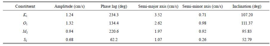
3 RESULT 3.1 Barotropic tideThe barotropic current ellipses for the four principal tidal constituents (K1, M2, O1, and S2) are plotted in Fig. 1, based on the harmonic results. All constituents, except for S2, were aligned with the cross-isobath direction. The semi-major axis of the ellipse for K1 was the largest, followed by those for O1 and M2. According to the harmonic constants of the four principal constituents listed in Table 1, the diurnal barotropic tides (K1 and O1) were the largest barotropic tidal constituents in this area. The amplitudes of u for K1 and O1 were comparable, as were the two D2 constituents (M2 and S2).
|
The internal tidal current ellipses of K1 and M2 were derived from the harmonic analysis of the baroclinic current data, as the representatives of D1 and D2, respectively (Fig. 3). It is obvious that the D1 current (K1) is much larger than the D2 current (M2). Moreover, the baroclinic current amplitudes of K1 and M2 were both larger than the barotropic counterparts, indicating that the baroclinic tide in this area is stronger than the barotropic tide. Generally, the K1 and M2 internal tides were shown to propagate in the northwest by west direction, but with an ambiguity of 180 °. This is consistent with other studies (Xu et al., 2011).

|
| Figure 3 Internal tidal ellipses at different depth for constituents K1(a) and M2(b) Black lines inside the current ellipses indicate the instantaneous currents at 10:00 local time (UTC+8)6 June 2011. Green lines indicate changes in current direction. |
In addition, there were some remarkable differences in vertical structure between the K1 and M2 constituents. The reversals of green lines in Fig. 3 indicate the general vertical structures for K1 and M2 internal tides.
Variations in the baroclinic current ellipse of K1 with depth show one current reversal, which is characteristic of the first-mode internal tide, in which two separate layers oscillate 180 ° out of phase with each other around 85 m. In contrast, the M2 presented a higher-mode structure with more oscillating layers around 40 m and 120 m.
3.2.2 Amplitude spectraFor convenience, only current data from the zonal component u were used for analysis in Sections 3.2.2 and 3.2.3. In Section 3.2.1, the magnitudes of ITD1(K1) and ITD2(M2) were preliminarily analyzed in terms of the baroclinic current ellipses. Amplitude spectra for the baroclinic velocity data at depths of 42 m and 202 m are shown in Fig. 4. The frequencies for D1 and D2 internal tides were 1 and 2 cycles per day, respectively. The spectra results confirm the preliminary analysis that ITD1 is dominant among the components. In addition, they provide additional information on these internal wave band peaks. There is no doubt that K1 and O1 were the two dominant components in the D1 frequency band, both at the surface (42 m) and the middle of the water column (202 m). Further, the scale of the K1 amplitude spectrum was greater than the O1 amplitude spectrum. In the D2 frequency band, S2 was the dominant component at the surface (42 m) and the amplitude spectrum of M2 was greater than the other D2 components in the middle of the water column (202 m). Another noteworthy feature was the largescale amplitude spectra at low frequency, indicating a strong barotropic flow in this area.

|
| Figure 4 Amplitude spectra for the velocity data at depths of (a)42 m and (b)202 m. D1 and D2 refer to 1 cycle per day and 2 cycles per day, respectively |
To better understand the vertical mode structures of the D1 and D2 internal tides, the baroclinic current data (for clarity, only the east-west velocity u is analyzed) were filtered by band-pass filters with frequency bands of Δf (D1)=[0.8, 1.2] and Δ f (D2)=[1.8, 2.2] cycles per day, respectively. The temporal and vertical variations of baroclinic velocity for ITD1 and ITD2 in the upper 200 m are presented in Fig. 5. In general, the magnitude of the D1 baroclinic current was larger than that of the D2 baroclinic current (note that the scales of the two images are different). This is consistent with the harmonic analysis. In most of the sample periods, the ITD1 took on a first-mode structure. In contrast, ITD2 seemed to exhibit a higher-mode structure. Moreover, there are some noteworthy and interesting patterns in the two images. For convenience, four rectangles are placed on both images (A-D).

|
| Figure 5 Time series (from 16 June to 26 July) of the filtered baroclinic current (u) data in the upper 200 m and the baroclinic velocity variances a. baroclinic current component u of ITD1 ; b. baroclinic current component u of ITD2 ; c. current variances of ITD1 ; d. ITD2 as a function of depth. The black rectangles indicate the periods analyzed in this paper. Note the different color scales between (a) and (b) and the different magnitudes for (c) and (d). |
Inside rectangle A (RA) in Fig. 5a, the magnitude of the baroclinic current for ITD1 was larger than those in the adjacent time periods. During this period, the obvious first-mode structure for ITD1 was captured, with two separate layers oscillating 180 ° out of phase and the transition occurring at 100 m depth. This phenomenon is consistent with the structure of the K1 current ellipse (Fig. 3a). Afterward, the ITD1 exhibited a third-mode structure, and a return to the first-mode structure on about 1 July 2011(RB). The left part of the RB shows the progress of the mode transformation (from third to first) for the vertical mode structure. In the right part of RB, ITD1 showed a first-mode structure similar to that in RA but the weak velocity cores were present at a lower depth of around 90 m. The mode structure subsequently transformed from the first to the second, and then from the second to the third (RC), indicating the transformation process from the first-mode to a higher-mode. Finally, the magnitude of baroclinic current for ITD1 reached a relatively high state between 12 July and 21 July (RD).
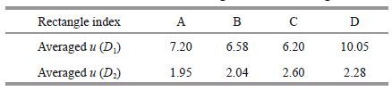
Table 2 lists the averaged baroclinic velocities for all rectangles. The ITD1 is clearly larger in RD than in the other three rectangles. The overall quasi-periodic temporal variation of the current values for ITD1 is shown, which is a signal for the spring-neap tide cycle. A similar phenomenon has been observed by other researchers (Liao et al., 2012 ; Xie et al., 2013). During most of the temporal series, the first-mode ITD1 currents dominated, and as a result, the overall D1 component (K1) showed a first-mode structure (Fig. 3a).
|
In contrast, the overall magnitude (Fig. 5b) of ITD2 was much smaller than ITD1(Fig. 5a). This is also consistent with the baroclinic current ellipses in Fig. 3. Inside the four rectangles, the mode structures and their temporal variations were too vague to be distinguished. Nevertheless, some signals of the firstmode (left side of RC and RD) and high-mode (left side of RA and right side of RD) structure could be seen. This phenomenon may explain the vertical structure formation of the baroclinic current ellipse of M2 in Fig. 3. For most of the time series, the ITD2 currents of high-mode were dominant, and as a result, the overall D2 component (M2) showed a high-mode structure.
To highlight the vertical structure, the variance of the baroclinic velocity was determined by integrating the spectrum over the D1 and D2 frequency bands (Fig. 5c, d). The magnitude of variance was much larger for ITD1 than ITD2, indicating a stronger movement in the D1 component than the D2 component. However, the two variances both appeared to depend on depth. The more energetic D1 component was maximal (144.6 cm 2 /s 2) near the surface of the observational range and minimal (47.6 cm2 /s2) in the middle of the water column. However, the less energetic D2 component also exhibited large variance, considering its small magnitude of baroclinic velocity. The variance for ITD2 with depth (Fig. 5d) was similar to that in Fig. 5c, with its maximum (17.7 cm 2 /s 2) near the surface and minimum (3.1 cm 2 /s 2) in the middle of the water column.
The dynamic mechanism for the temporal transformation for the multimodal IT in this area is still not understood. However, some studies have used numerical models to investigate these mechanisms. Vlasenko et al.(2010) indicated that during the progress of wave propagation, several types of baroclinic waveforms can be generated in the course of its disintegration. A group of waves has the greatest phase speed, and therefore detaches quickly from the wave tail and propagate independently. Thus, a variety of modal structures will appear in the baroclinic current field. Xu et al.(2011) presented some tentative hypotheses for the transformation of IT modal structures. First, changes in stratification, background shear and significant nonlinear bottom drag may alter the modal content from low to higher modes (St. Laurent and Garrett, 2002 ; Nash et al., 2004). Second, internal tides are dependent on local stratification. Factors contributing to the structure of the internal tides also include stratification variations at the deep generation sites, mesoscale activity and the shoaling of a random internal wave field.
3.2.4 Empirical Orthogonal Function (EOF) analysisThe method of empirical EOF analysis is by decomposition of a data set that finds both spatial patterns and temporal variations. In this section, EOF analyses of the zonal currents u were applied to reveal the detailed multimodal structure of IT. To be consistent with the analyses in section 3.2.3, only current data in the upper 200 m were used for EOF analyses. Moreover, to study the temporal variation of the modal structures for ITD1 and ITD2, the EOF analyses were performed on weeklong data sets. Figures 6 -8 present the modal structures and amplitude spectral of temporal variances for the first three EOF modes in weeks 1, 3, and 8, respectively. The amplitude spectra represent the modal structures of ITs at different frequencies. Table 3 lists the percentages of the total variances for the first three EOF modes during weeks 1, 3, and 8.

|
| Figure 6 EOF analysis of zonal baroclinic currents u in week 1 a. vertical structure of first three baroclinic modes; b. amplitude spectral of the eigenfunction time series for first three modes. |

|
| Figure 7 EOF analysis of zonal baroclinic currents u in week 3 a. vertical structure of first three baroclinic modes; b. amplitude spectral of the eigenfunction time series for first three modes. |

|
| Figure 8 EOF analysis of zonal baroclinic currents u in week 8 a. vertical structure of first three baroclinic modes; b. amplitude spectral of the eigenfunction time series for first three modes. |
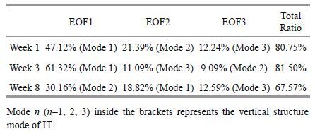
The temporal variance in the modal structures for both ITD1 and ITD2 was easily identified from the analysis results. During weeks 1 and 3, the first three EOF modes contributed more than 80% of the total variances. The mode-1 IT was predominant in the D1 frequency band, which matches the descriptions in Section 3.2.3. In the D2 frequency band, the amplitude spectra for the first three EOF modes were all smaller than those in the D1 frequency band. This indicates that the magnitude of ITD2 was much smaller than ITD2, which is also consistent with the previous description. Nevertheless, there were obvious differences between EOF analysis results in week 1 and week 3. The contribution percentages of the mode-1 and mode-2 ITs both underwent significant changes from weeks 1 to 3. The mode-1 IT accounted for more than half (61.32%) of the total variance in week 3, while the percentage in week 1 was only 47.12%. This means that 14.2% of mode-1 IT had transferred to higher-mode motions. The modal structure of the first-mode diurnal component in Fig. 7 displayed a reversal layer in the vertical, with a zero crossing point at 110 m depth. This is in qualitative agreement with the contours of the diurnal zonal currents in rectangle A (Fig. 5a ; oscillating layers around 110 m). In addition, the contribution percentage of mode-2 IT decreased by 12.3% from weeks 1 to 3. In short, the results of EOF analysis in weeks 1 and 3 clearly revealed the transformation between different multimodal structures of IT.
The EOF analysis in week 8 revealed interesting differences. Figure 8 indicates that EOF results in week 8 were completely different from those in weeks 1 and 3. The first three EOF modes only contributed 67.57% of the total variances, which is smaller than the percentages in weeks 1 and 3. This is evidence that, during week 8, there were more high-mode motions compared with the other two weeks. Moreover, the mode-2 IT dominated the whole zonal current field, but failed to dominate in the D1 and D2 frequency bands. The first three mode motions of IT had comparable magnitudes in the D1 and D2 frequency bands.
3.2.5 Kinetic energy of coherent internal tideTo better understand the relative importance of the four main tidal constituents, we decomposed the current data into coherent and incoherent components using results from harmonic analysis. The coherent component was obtained from
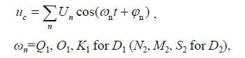 (1)
(1)where Un is the amplitude of the n -th constituent and φ n is its phase. The incoherent IT component was then defined as
 (2)
(2)Figure 9 shows the coherent kinetic energy (hereafter referred to as KEC and KEC = u c 2 + v c 2) of the different components. All the KEC values in the upper 200 m show approximate fortnightly spring-neap cycles, which is consistent with the phenomenon found in Fig. 5. As plotted in Fig. 9a, the correlation coefficient between KEC D1+ D2 and KEC D1 is 0.84, which means the two series are highly correlated. Thus, from the perspective of KEC, ITD1 dominated the IT field. The correlation coefficients for the time series in Fig. 9b and 9c are 0.91 and 0.90, respectively, both showing high correlations. The high correlation shows that the diurnal 14-day cycle was induced by the superposition of O1 and K1(Fig. 9b), while the semidiurnal 14-day cycle was mainly induced by the superposition of M2 and S2(Fig. 9c)(Xie et al., 2013). However, there was a significant variation in D2 spring tides. The largest KEC D2 appears on 8 July 2011, having a significant shift with respect to the peak of the coherent M2 + S2 signals. The above shift is partly due to the modulation of other coherent constituents, such as N2. Alternatively, the shift may be due to the effect of the varying background conditions (van Haren, 2004).

|
| Figure 9 KEC of different components Note the different magnitudes for (b) and (c). |
A 71-day ADCP velocity time series from the continental slope near the Dongsha Plateau was examined to study the temporal variability in internal tides in the northern South China Sea. Results of harmonic and spectra analysis indicate that the diurnal internal tide was overwhelmingly dominant in this area. We also presented evidence of the multimodal semidiurnal internal tide and showed that the firstmode signals dominated diurnal variations in the northern SCS. The band-filtered data set for ITD1 revealed fortnightly variations, while the dataset for ITD2 was too vague to distinguish the variation period. The time variation of current data for ITD1 and ITD2 showed the vertical transformations for the two kinds of internal tides. For the ITD1 current data, the modeone structure generally dominated the time variations for most of the time. Nevertheless, the vertical mode structure for ITD1 cycled from mode-one to higher modes and back to mode-one again. As for the current data of ITD2, the cycle for the vertical mode structure was not clear because of the small velocity and overall complex mode structure. The results of EOF analyses during the different weeks revealed detailed temporal variations in multimodal structures for ITD1 and ITD2. The EOF results were consistent with the conclusions obtained above. Generally, ITD1 exhibited a first-mode vertical structure, which may transform between lowmode and high-mode in some circumstances. In contrast, although with smaller current magnitude, ITD2 presented more complex vertical structures than ITD1 during most of the study period. The first three baroclinic modes of ITD2 had comparable magnitudes during the study period. The KEC of ITD1 was about ten times greater than ITD2, which is consistent with the discussions in the previous sections and other studies (Ma et al., 2013 ; Xie et al., 2013).
| Alford M H, 2003. Redistribution of energy available for ocean mixing by long-range propagation of internal waves. Nature, 423 (6936) : 159 –162. Doi: 10.1038/nature01628 |
| Alford M H, 2008. Observations of parametric subharmonic instability of the diurnal internal tide in the South China Sea. Geophysical Research Letters, 35 (15) : L15602 . Doi: 10.1029/2008GL034720 |
| Duda T F, Lynch J F, Irish J D, Beardsley R C, Ramp S R, Chiu C S, Tang T Y, Yang Y J, 2004. Internal tide and nonlinear internal wave behavior at the continental slope in the northern South China Sea. IEEE Journal of Oceanic Engineering, 29 (4) : 1105 –1130. Doi: 10.1109/JOE.2004.836998 |
| Duda T F, Rainville L, 2008. Diurnal and semidiurnal internal tide energy flux at a continental slope in the South China Sea. Journal of Geophysical Research, 113 (C3) : C03025 . |
| Fang G H, Kwok Y K, Yu K J, Zhu Y H, 1999. Numerical simulation of principal tidal constituents in the South China Sea, Gulf of Tonkin and Gulf of Thailand. Continental Shelf Research, 19 (7) : 845 –869. Doi: 10.1016/S0278-4343(99)00002-3 |
| Floor J W, Auclair F, Marsaleix P, 2011. Energy transfers in internal tide generation, propagation and dissipation in the deep ocean. Ocean Modelling, 38 (1-2) : 22 –40. Doi: 10.1016/j.ocemod.2011.01.009 |
| Garrett C, Kunze E, 2007. Internal tide generation in the deep ocean. Annual Review of Fluid Mechanics, 39 (1) : 57 –87. Doi: 10.1146/annurev.fluid.39.050905.110227 |
| Helfrich K R, Melville W K, 2006. Long nonlinear internal waves. Annual Review of Fluid Mechanics, 38 (1) : 395 –425. Doi: 10.1146/annurev.fluid.38.050304.092129 |
| Jan S, Chern C S, Wang J, Chao S Y, 2007. Generation of diurnal K1 internal tide in the Luzon Strait and its influence on surface tide in the South China Sea. Journal of Geophysical Research: Oceans, 112 (C6) : C06019 . |
| Klymak J M, Alford M H, Pinkel R, Lien R C, Yang Y J, Tang T Y, 2011. The breaking and scattering of the internal tide on a continental slope. Journal of Physical Oceanography, 41 (5) : 926 –945. Doi: 10.1175/2010JPO4500.1 |
| Lee I H, Wang Y H, Yang Y, Wang D P, 2012. Temporal variability of internal tides in the northeast South China Sea. Journal of Geophysical Research: Oceans, 117 (C2) : C02013 . |
| Liao G H, Yuan Y C, Yang C H, Chen H, Wang H Q, Huang W G, 2012. Current observations of internal tides and parametric subharmonic instability in Luzon Strait. Atmosphere-Ocean, 50 (S1) : 59 –76. |
| Lien R C, Tang T Y, Chang M H, D'Asaro E A, 2005. Energy of nonlinear internal waves in the South China Sea. Geophysical Research Letters, 32 (5) : L05615 . |
| Liu J L, Cai S Q, Wang S, 2010. Currents and mixing in the northern south china sea. Chinese Journal of Oceanology and Limnology, 28 (5) : 974e980 . |
| Locarnini R A, Mishonov A V, Antonov J I et al. 2006. World ocean atlas 2005 Volume 1: temperature. In: Levitus S ed. NOAA Atlas NESDIS 61. U.S. Government Printing Office, Washington D C. |
| Ma B B, Lien R C, Ko D S, 2013. The variability of internal tides in the Northern South China Sea. Journal of Oceanography, 69 (5) : 619 –630. Doi: 10.1007/s10872-013-0198-0 |
| Moum J N, Caldwell D R, Nash J D, Gunderson G D, 2002. Observations of boundary mixing over the continental slope. Journal of Physical Oceanography, 32 (7) : 2113 –2130. Doi: 10.1175/1520-0485(2002)032<2113:OOBMOT>2.0.CO;2 |
| Nash J D, Kunze E, Toole J M, Schmitt R W, 2004. Internal tide reflection and turbulent mixing on the continental slope. Journal of Physical Oceanography, 34 (5) : 1117 –1134. Doi: 10.1175/1520-0485(2004)034<1117:ITRATM>2.0.CO;2 |
| Niwa Y, Hibiya T, 2001. Numerical study of the spatial distribution of the M2 internal tide in the Pacific Ocean. Journal of Geophysical Research: Oceans, 106 (C10) : 22441 –22449. Doi: 10.1029/2000JC000770 |
| Niwa Y, Hibiya T, 2004. Three-dimensional numerical simulation of M2 internal tides in the East China Sea. Journal of Geophysical Research: Oceans, 109 (C4) : C04027 . |
| St. Laurent L, Garrett C, 2002. The role of internal tides in mixing the deep ocean. Journal of Physical Oceanography, 32 (10) : 2882 –2899. Doi: 10.1175/1520-0485(2002)032<2882:TROITI>2.0.CO;2 |
| Sun O M, Pinkel R, 2013. Subharmonic energy transfer from the semidiurnal internal tide to near-diurnal Motions over Kaena Ridge, Hawaii. Journal of Physical Oceanography, 43 (4) : 766 –789. Doi: 10.1175/JPO-D-12-0141.1 |
| van Haren H, 2004. Incoherent internal tidal currents in the deep ocean. Ocean Dynamics, 54 (1) : 66 –76. Doi: 10.1007/s10236-003-0083-2 |
| Vlasenko V, Stashchuk N, Guo C, Chen X, 2010. Multimodal structure of baroclinic tides in the South China Sea. Nonlinear Processes in Geophysics, 17 (5) : 529 –543. Doi: 10.5194/npg-17-529-2010 |
| Xie X H, Shang X D, Chen G Y, Sun L, 2009. Variations of diurnal and inertial spectral peaks near the bi-diurnal critical latitude. Geophysical Research Letters, 36 (2) : L02606 . |
| Xie X H, Shang X D, van Haren H, Chen G Y, 2013. Observations of enhanced nonlinear instability in the surface reflection of internal tides. Geophysical Research Letters, 40 (8) : 1580 –1586. Doi: 10.1002/grl.50322 |
| Xu Z H, Yin B S, Hou Y J, Xu Y, 2013. Variability of internal tides and near-inertial waves on the continental slope of the northwestern South China Sea. Journal of Geophysical Research-Oceans, 118 (1) : 197 –211. Doi: 10.1029/2012JC008212 |
| Xu Z H, Yin B S, Hou Y J, 2011. Multimodal structure of the internal tides on the continental shelf of the northwestern South China Sea. Estuarine, Coastal and Shelf Science, 95 (1) : 178 –185. Doi: 10.1016/j.ecss.2011.08.026 |
| Yang Y J, Tang T Y, Chang M H, Liu A K, Hsu M K, Ramp S R, 2004. Solitons northeast of Tung-Sha Island during the ASIAEX pilot studies. IEEE Journal of Oceanic Engineering, 29 (4) : 1182 –1199. Doi: 10.1109/JOE.2004.841424 |
| Zhao Z X, Klemas V, Zheng Q N, Yan X H, 2004. Remote sensing evidence for baroclinic tide origin of internal solitary waves in the northeastern South China Sea. Geophysical Research Letters, 31 (6) : L06302 . |