 2017, Vol. 35
Institute of Oceanology, Chinese Academy of Sciences
Article Information
- YU Kun(于堃), JI Guangrong(姬光荣), ZHENG Haiyong(郑海永)
- Automatic cell object extraction of red tide algae in microscopic images
- Chinese Journal of Oceanology and Limnology, 35(2): 275-293
- http://dx.doi.org/10.1007/s00343-016-5324-6
Article History
- Received Nov. 5, 2015
- accepted in principle Jan. 8, 2016
- accepted for publication Feb. 19, 2016


Harmful algal blooms (HABs) are a worldwide marine environmental issue and ecological disaster. The species of red tide algae directly determines the extent of the damage of algal blooms, so quick and valid identification of red tide algae is of considerable importance for the monitoring and early warning of HABs. The traditional identification measure requires experts to observe the algae’s morphology with the aid of a microscope to implement classification, which requires high levels of professional knowledge and experience. It is also time-consuming and laborious. In recent years, with the development of in situ optical imaging systems (Erickson et al., 2012), the microscopic image analysis of algae through computer vision technology (Culverhouse et al., 2006) has received increasing attention, as it allows both real-time analysis and a large throughput.
Precise and efficient extraction of cell objects from microscopic images is essential for algae analysis, and is an indispensable part of automatic microscopic image recognition systems for HABs. Jalba et al. (2004) proposed an improved watershed algorithm that is controlled by connected operator markers to segment diatom cells in microscopic images. This approach significantly improved the initial segmentation results of the automatic diatom identification and classification project (Fischer et al., 2002), and has been applied to the classification system of diatom images (Dimitrovski et al., 2012). Blaschko et al. (2005) used a snake-based method to generate contours and an intensity-based method to determine the details of plankton images collected by a flow imaging instrument. Rodenacker et al. (2006) adopted a threshold strategy to segment plankton cells in microscopic images, whereas Sosik and Olson (2007) combined threshold-based edge detection with phase congruency to extract the features of phytoplankton cells. Luo et al. (2011) used a regression method and Canny edge detection for segmentation calibration to search for circular diatoms in microscopic images, and Verikas et al. (2012) segmented the circular Prorocentrum minimum cell objects from microscopic images using a fuzzy C-means clustering algorithm.
Most of these studies used a single edge-based (i.e., Canny) or region-based (i.e., threshold and clustering) method to segment several particular species of algae. These approaches can easily result in under-or over-segmentation for other species of algae with different morphological characteristics.
In microscopic images of red tide algae, algal cells are typically translucent and small (usually micron level), and have fuzzy boundary shadows and complex structural characteristics. The cells often survive as a monomer or chain group. When a micrograph is captured, background areas consisting of culture fluid or seawater are usually compounded by cellular debris, silt and other impurities. These may lead to random noise. Moreover, the free movement of algae can produce water vortex (water stain) noise around the algae. Additionally, unreasonable microscopy, especially inappropriate brightness of the microscope light source, often leads to micrographs that have uneven illumination, low contrast, and even vague cell objects.
By observing and analyzing the biological morphological characteristics of algae, we found that certain species possess subtle setae on the main chain that are obviously different from other species. These algae with setae can cause red tide, and are generally of the Chaetoceros strain. Therefore, we roughly divide red tide algae into two categories, non-setae algae species and Chaetoceros, and design appropriate segmentation strategies to extract cell objects from each type.
Human-computer interactive methods make the segmentation effect more precise owing to the intervention of human subjective factors. A representative algorithm is GrabCut (Rother et al., 2004). Based on graph cut theory, GrabCut has become popular because of its simple interactivity and excellent segmentation effect. However, this algorithm has obvious shortcomings: it requires the foreground and background to be manually labeled, and can only extract a single object.
We consider the human visual system to be involved in the process of microscopic imaging. If we can automatically initialize GrabCut through visual attention and superimpose multiple single-object segmented images, then the above problems will be overcome.
Saliency maps can reflect the degree of stimulation that an image causes in the human eye. Ideally, image acquisition will only be carried out when algal cells appear in the microscopic. As the higher saliency of cell regions causes more visual stimulation to the human eye, it is reasonable to take advantage of saliency maps to establish the initial segmentation markers.
For non-setae algae, we propose a non-interactive GrabCut method combined with salient region detection to automatically segment both unicellular and multicellular objects. We first construct a multiscale salient region detection system based on the border-correlation of superpixels to locate cell regions. We then use some morphological operations to obtain the pre-segmented result as the initial mask image. The GrabCut algorithm is then initialized by the mask image and the rectangular window, and GrabCut is executed iteratively. Finally, big contour extraction and median filtering are carried out in turn to remove noise and smooth the boundary, respectively. Note that we introduce the area-ratio threshold and similarity detection in the segmentation process to exclude those pseudo-cell regions that are conspicuous but do not actually contain cells.
For Chaetoceros, as its setae have such a light color and low contrast with the background, the the current mainstream segmentation methods cannot validly determine the setae. Hence we present a method based on the gray surface orientation angle model to extract the cells containing setae. This method first builds a gray surface vector model using knowledge of the space vector, and then conducts gray mapping of the orientation angle. The obtained gray values are reconstructed in the xz-and yz-planes. Ultimately, we carry out morphological processing to preserve the setae information and eliminate the noise interference.
A series of experiments verify the effectiveness of our proposed methods.
2 MICROSCOPIC IMAGE ACQUISITIONMost of the algal specimens studied in this paper are kept in the Key Laboratory of Marine Environment and Ecology of the Ministry of Education at Ocean University, and the Research Center for Harmful Algae and Aquatic Environment at Jinan University, both in China. These specimens are collected from the frequent HABs occurrences in the East China Sea and the South China Sea, and the corresponding microscopic images (optical micrographs) of algal cells are captured by Olympus BX series optical microscopes (Olympus Corporation, Tokyo, Japan) with the high-sensitivity, high-speed professional micrography system QImaging Retiga 4000R FAST 1394 CCD (QImaging Corporation, Surrey, Canada).
Other parts of the algal specimens are sampled at sea by the R/V Dong Fang Hong 2, and the corresponding microscopic images of algal cells are captured by Nikon Eclipse E800 microscopes with a micrography system consisting of a CFI60 optical instrument and the Nikon Digital Sight camera (Nikon Corporation, Tokyo, Japan), controlled by Image Pro Plus software (Media Cybernetics Incorporated, Rockville, Maryland, USA).
Using the optical microscope equipped with this micrography system to acquire algal cell images includes two main steps: sampling and imaging.
2.1 Sampling1. Before sampling, it is necessary to gently shake the container (normally a test-tube) holding the algal sample, so as to disturb the sample. A pipettor is then used to extract 100 μL from the container and place the liquid on a clean glass slide. Note that some algae species (such as Alexandrium catenella) are extremely prone to deformation under extrusion of the cover glass, making it necessary to take a smaller amount of liquid (about 70 μL).
2. Place the glass slide onto the mobile microscope stage and adjust the x/y axis knob so that the observation objects enter the optical path of the objective lens.
3. Cover the glass slide with the cover glass.
2.2 Imaging1. Observe and select the specific cell objects with in the visual field through the eyepiece.
2. Select the specific imaging technology, typically bright field (BF) or differential interference contrast (DIC) mode. BF is mainly used for the observation of stained specimens, whereas DIC is mainly used for the observation of transparent specimens and emphasizes three-dimensional effects.
3. Open the micrography control software on the computer, and adjust the control parameters and take pictures by manipulating the computer. Finally, the captured images are named and saved digitally.
Note that sampling changes the living environment of algae species considerably (primarily in terms of temperature and light). Some algae species (such as Chattonella marina) are very prone to cell autolysis after a short time, which means the cells destroy themselves by the activity of a digestive enzyme. Therefore, the micrographs must be captured quickly. If necessary, repeated sampling and observations must be carried out at different magnifications.
3 NON-SETAE ALGAL CELL SEGMENTATION 3.1 Algal cell region detectionFigure 1 displays the detailed procedures involved in the detection of non-setae algal cell regions. We first define the border-correlation at the superpixel level, and then extend this to a saliency calculation based on the color contrast. The generated saliency values are optimized. Finally, the saliency maps produced under multiple scales are merged into one map as the final detection result.

|
| Figure 1 Flow chart of the non-setae algal cell region detection algorithm. The alga in the diagram is Gonyaulax polygramma |
The photographer will usually places the algal cells in the middle (away from the edges) of the picture being captured. Thus, we use a border-correlation measure (referred to as the BC method) to distinguish the algal cell from background regions: when a region is closely related to the border, it is thought to be a background region; otherwise, it is an algal object.
In particular, we first adopt a soft segmentation method called Simple Linear Iterative Clustering (SLIC) (Achanta et al., 2012), to divide the input image into M regular and compact superpixels. Each superpixel {ai} (i=1, 2, …, M) is composed of a fixed number of pixels, which can better reflect the local structural information. The number of superpixels along the border of the image is N, and each border superpixel is expressed as {bj}, j=1, 2, …, N.
We construct an undirected graph G=(V, E, T), where V is a set of the virtual superpixel nodes; E is a set of two kinds of undirected edges: internal edges, which connect all adjacent superpixels, and border edges, which link any two border superpixels; T is a set of weights that belong to the edges. The weight W(ap, aq) of the edge connecting superpixels ap and aq (if p=q, W(ap, aq)=0) is defined as the Euclidean distance between their respective average colors in the CIE-Lab color space.
Inspired by the geodesic saliency (Wei et al., 2012), the geodesic distance between any two superpixels can be computed by adding the edge weights along their nearest connected route in G:
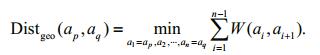 (1)
(1)The degree of relatedness between superpixel ai and the border region is further derived as:
 (2)
(2)where Ck (k=1, 2, 3, 4) is a negative adjustment coefficient. The values of exp (•) range from 0 to 1. If the two regions containing ai and bj have a similar color, then Distgeo(ai, bj)≈0, exp (•)≈1. This means ai is closely connected to the border superpixel bj. Conversely, when Distgeo(ai, bj)≈1, we can assume that there is no relationship between ai and bj.
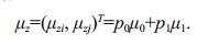
Similar to the above definition, the degree of relatedness between superpixel ai and the whole image is:
 (3)
(3)Considering the above, the border-correlation of superpixel ai can be defined by the ratio:
 (4)
(4)This quantity specifically describes the extent of the connection between a superpixel and the image border. When a superpixel is on the object, its bordercorrelation is much smaller than when it is located on the background.
3.1.2 Saliency calculationThe border-correlation is an effective measure of whether a superpixel is on the object region, but does not, on its own, highlight the algal cells from the background.
A valid solution is to extend the border-correlation to the saliency calculation. Referring to the definition of a pixel’s contrast saliency (Cheng et al., 2011), superpixel ai’s saliency value can be defined by its color contrast with respect to other superpixels in the image. This is implemented by computing the weighted sum of ai’s color distance to the other superpixel regions in the CIE-Lab color space:
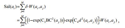 (5)
(5)where the weight δ consists of a background probability weighting term (1-exp (C3BC2(aj))) and a spatial weighting term exp (C4 d2(ai, aj)). In addition, d(ai, aj) denotes the Euclidean spatial distance between the centroids of superpixel regions ai and aj. Note that Sal (ai) is assigned to all of the pixels contained in ai.
Regardless of whether ai belongs to a salient object or the background, we assume that aj is part of the salient object. Thus, aj’s border-correlation will be very small (close to 0), so its background probability will be approximately 0. This means that aj makes only a small contribution to ai’s saliency value. On the contrary, if aj belongs to the background, its background probability converges to 1, and it will contribute much more to ai’s saliency value.
Overall, introducing the background probability strengthens the contrast in the salient object superpixels while weakening the contrast in the background superpixels. This approach significantly expands the difference between the saliency values of the salient object and the background, which assists the preliminary separation of the object from the background.
Unfortunately, however, the dividing line between the salient object and the background is fuzzy, and the saliency map contains excessive irregular noise. Thus, it is necessary to optimize the saliency map.
3.1.3 Optimization of saliency mapMost existing methods employ Gaussian filtering or other types of filters, such as a guided filter (He et al., 2010), to smooth the saliency map. However, this process can lead to the loss of visual clarity and resolution. In our work, to avoid blurring the images, we adopt a simple but effective technique in which all the saliency values are normalized to [0, 1], and two thresholds are set to divide all the superpixels into three categories:
(1) The superpixels with background probabilities larger than the high threshold are assigned a saliency value of 0.
(2) The superpixels with background probabilities smaller than the low threshold are assigned a saliency value of 1.
(3) The remainder of the superpixels retain their original saliency values.
Through these steps, we obtain optimized saliency maps that approximate to binary images. The white regions correspond to the first category of superpixels and are thereby considered to be salient objects. The black regions represent the background specified by the second kind of superpixel. Given the limitations of salient object detection, there exist a small number of gray regions that include the uncertain third type of superpixel, which are neither object nor background.
3.1.4 Fusion of multi-layer saliency mapsThe saliency maps described above are generated by the basic units of superpixels, so the selection of the number of superpixels plays a decisive role in the accuracy of the saliency maps. If we specify the same number of superpixels in advance, it is very difficult to apply this approach to various species of non-setae algae images.
Therefore, we adopt a flexible strategy of multiscale fusion that is robust to changes in the shape and size of algal cells. First, three layers of superpixellevel saliency maps are generated. In each layer, the number of pixels in each superpixel is specified to be 150, 200 and 250, respectively. This ensures that the actual number of superpixels is proportional to the total number of pixels in the input image. We then compute the arithmetic average of the saliency values of the three layers, and linearly stretch these values as the final saliency values for enhancing the contrast of the saliency maps.
3.2 Automatic extraction of algal cellsIn this section, we first describe the presegmentation of the saliency map and then explain the dual initialization of GrabCut with both the presegmented result and the rectangular window, which avoids the need for human-computer interaction. In addition, multi-object segmentation is realized by means of superimposing multiple single-object segmented results. Figure 2 shows the cell extraction process.

|
| Figure 2 Extraction process of non-setae algal cells based on non-interactive GrabCut |
In some saliency maps, the contour line of the cell body is broken. If we directly segment these maps, some important components of the cell will undoubtedly be lost. Therefore, we first morphologically dilate the saliency map.
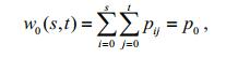
To ensure that object regions can be fully separated, it is necessary to choose one threshold segmentation method to realize saliency map binarization. Obviously, a fixed threshold cannot be appropriate for all saliency maps. We introduce a two-dimensional (2D) Otsu method based on a 2D histogram to adaptively determine the optimal threshold. Unlike the usual one-dimensional (1D) Otsu method (Otsu, 1979), our technique reflects not only the gray level distribution but also the spatial distribution information of pixels, providing stronger noise immunity even if the signal-to-noise ratio of the image is low. The algorithm proceeds as follows:
(1) The first step is to construct a 2D histogram. For an M×N image, let f(x, y) represent the gray value of pixel (x, y), and g(x, y) represent the average gray value of a 3×3 square neighborhood centered on (x, y). Both f(x, y) and g(x, y) have the same gray level L and constitute a 2D vector (i, j). cij indicates the number of times that (i, j) appears. Supposing that pij is the occurrence frequency of (i, j), we have that pij=cij/(M×N). Thus, the 2D histogram is defined in a square region with side length L (set to 256), and has X-, Y-, and Z-coordinates of i, j, and pij, respectively. The 2D histogram of the Ceratium tripos saliency map after dilation is shown in Fig. 3.

|
| Figure 3 2D histogram of morphological dilated saliency map for Ceratium tripos |
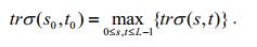
(2) If we take a threshold vector (s, t), 0≤s, t≤L-1, then the definition domain of the 2D histogram (shown in Fig. 4) is divided into four regions. Region 1 corresponds to the background, Region 3 corresponds to the object, and Regions 2 and 4 correspond to a small number of uncertain pixels near the contour.

|
| Figure 4 Definition domain of 2D histogram |
(3) The occurrence probabilities of the object and the background are respectively:
 (6)
(6) (7)
(7)(4) The gray mean vectors of the object and the background can be calculated, respectively, as:
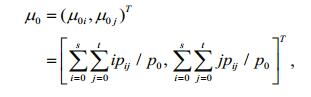 (8)
(8)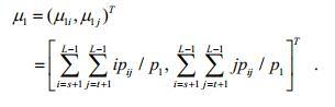 (9)
(9)The number of pixels near the contour is much lower than the total number of pixels in the whole image. We assume that pij is approximately 0 in Regions 2 and 4, so these regions can be ignored. Thus, the total gray mean vector of the whole image is:
 (10)
(10)(5) The Discrete Measure Matrix between the object and the background is defined as:
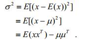
 (11)
(11)The trace (sum of all elements on the main diagonal) of the matrix σ is treated as the Distance Measure Function between the object and the background:
 (12)
(12)The gray difference between the object and the background is greatest when the trace attains a maximum. The corresponding threshold vector (s0, t0) is the optimal threshold vector for the binarization of the saliency map.
 (13)
(13)Subsequently, the morphological close operation is carried out to remove small holes and cracks in the binary images.
Empirically, the maximum distinguishable object must be seaweed in the actual micrographs. Therefore, to eliminate speckle noise, we only extract the contour of the largest connected region (with area Smax) and those contours whose enclosed area is greater than or equal to 30% of Smax, and then fill the interior regions of these contours with white. At this point, morphological erosion is used to shrink the large foreground areas to make them close to the actual size. The process of pre-segmentation is illustrated in Fig. 5b-f.

|
| Figure 5 Automatic extraction pipeline of non-setae algal cells a. original microscopic images; b. morphological dilation for saliency maps; c. threshold segmentation; d. morphological close; e. big contours extraction; f. pre-segmentation results after morphological erosion; g. rectangular windows initialization; h. mask images after GrabCut execution; i. repeated big contours extraction. From top to bottom: Prorocentrum sigmoides, Gonyaulax spinifera, Gymnodinium catenatum, Ceratium tripos, Prorocentrum minimum and Pleurosigma affine. |
GrabCut is a supervised segmentation algorithm proposed by Carsten et al. on the basis of Graph Cuts (Boykov and Jolly, 2001). This algorithm requires the manual labeling of some foreground and background pixels as the seed points to establish the respective color models. The input image is then mapped to a directed graph. The optimal solution of the directed graph is solved using the max-flow/min-cut method.
For simple images, we can achieve good segmented results with a small number of markers. However, for complicated algae microscopic images, it is necessary to add many markers, and the segmentation accuracy can be extremely poor if there are too fewmarkers or if they are poorly positioned.
In this paper, we use and optimize the GrabCut algorithm to avoid this tedious marking process and make it suitable for the extraction of algal cells.
3.2.2.1 Algorithm initializationInitialization generally refers to providing indicative cues for the algorithm via human-computer interaction to guide the segmentation. For the huge number of microscopic algae images, the single interaction mode does not work. Moreover, the efficiency of manual input is so low that real-time segmentation and automatic batch processing cannot be achieved. This paper describes the use of both a mask image and rectangular window to automatically initialize GrabCut, instead of the usual humancomputer interaction. We refer to this as “noninteraction” mode.
Specifically, the pre-segmented binary results that contain rich location information about the pixels can be directly used to define the initial mask image. The mask image is a single-channel grayscale image that has the same size as the source image, and each pixel of the mask image can only take four kinds of enumerated values: “background”, “foreground”, “probable background” and “probable foreground”. We set the white and black regional pixels of the binary image to “probable foreground” and “background”, respectively. The mask image is used to constrain the segmentation during the execution of GrabCut.
To initialize the rectangular window, we first calculate the bounding box of the foreground object in the pre-segmented result. The bounding box is defined as the minimum enclosing rectangle that includes the object and whose sides are parallel to the coordinate axis, which closely describes and displays the range of the connected region corresponding to the object. Through a line-by-line traversal of the binary image, we can identify the four tangent points of the object contour that lie along the coordinate axis direction. With the coordinates of these four points, the location and size of the bounding box can be computed. Expanding the bounding box slightly determines the rectangular window. The region outside the window is defined as background, whereas the region inside the window is defined as probable foreground.
In addition, as the micrographs considered here are taken by high-resolution microscopic imaging equipment, they have a large size. Thus, we carry out down-sampling of the input image to reduce the computational complexity.
3.2.2.2 Suspicious cell region detectionWhen many cells appear in the images, they generally belong to the same category of algae. Similarity detection can rule out those pseudo cell regions and confirm the sequence number and quantity of the real cell regions. The largest connected region is regarded as the reference region, as it must be a cell region.
We first adjust all the regions to have the same size as the smallest region, and then detect the similarity between each region and the reference region by comparing their respective histograms. The similarity is defined as the ratio of the number of similar pixels to the total number of pixels in the reference region.
When the similarity between a candidate region and the reference region reaches some minimum requirement (set to 75%), the candidate is identified as a true cell region. Otherwise, it is considered to be a false cell region, and we remove its rectangular window and update the pixels of this region in the mask image to “background”. Figure 6 illustrates the detection process.

|
| Figure 6 Similarity detection for Amphidinium carterae a. original microscopic image; b. saliency map; c. pre-segmentation result before morphological erosion; d. pre-segmentation result; e. initial rectangular window. The rectangular region on the left is used as the reference region. The similarities of the rectangular regions above and on the right of the reference region are 63.53% and 87.03%, respectively; f. updated rectangular window; g. final segmentation result. |
After initializing the algorithm, it is necessary to create a Gaussian Mixture Model (GMM) that can describe the foreground and background according to the marker information, and update this model in the iterative process.
In RGB color space, assuming an arbitrary pixel in an image is x=(r, g, b)T, the probability density function of the Single Gaussian Model (SGM) is:
 (14)
(14)where μ and σ2 denote the mean value and variance, respectively, and are calculated as follows:
 (15)
(15) (16)
(16)The GMM can be expressed as the weighted probability density sum of n SGMs:
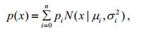 (17)
(17)where pi is the weight of SGM i.
The GMM represents the characteristics of each pixel in the image. The weight of each SGM is an important parameter that denotes the proportion of the SGMs that contribute to the whole GMM.
To build a GMM containing n SGMs, the image must be divided into n categories, and each category must be fitted to an SGM whose weight is equal to the ratio of this category’s number of pixels to the total number of pixels. We use the K-means clustering algorithm for image classification, as this continuously optimizes the classification results in each iteration.
The labeled pixel sets B and U of the background and probable foreground, respectively, can be used to train the GMM of the background and foreground.
3.2.2.4 Gibbs energy functionThe image with marker information is mapped to a directed graph, and the regional and border performance of this directed graph can be described by the Gibbs energy function:
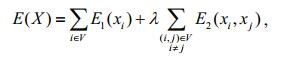 (18)
(18)where xi and xj are the label values of nodes i and j (1 for foreground and 0 for background); E1 is the similarity energy, which denotes the similarity between each pixel and the foreground or background; E2 is the priority energy, which denotes the similarity between adjacent pixels.
Because each GMM can be regarded as a K-dimensional covariance, the vector k=(k1, …, kn, …, kN) is introduced as the independent GMM parameter of each pixel, where kn∈{1, 2, …, K}. Thus, the Gibbs energy function can be rewritten as:
 (19)
(19)where α is the opacity distribution (α∈[0, 1]), where α=0 corresponds to the background and α=1 corresponds to the foreground; θ is the gray histogram of the foreground and background, θ={h(z, α), α=0, 1}; z is the gray value array, z=(z1, …, zn, …, zN).
When the Gibbs energy function attains a minimum, we set the weights on the edges of the directed graph according to the relationship between the region and the boundary, thus transforming the image segmentation problem into the dichotomy problem of directed graphs. Therefore, the optimal segmented image is obtained by determining the optimal solution of the directed graph with the max-flow/min-cut method.
After executing the GrabCut algorithm, we obtain a single-object segmented image. Using the logical “or” operation for the multiple single-object segmented images, we can further obtain a multiobject segmented image. We then extract the big contours and fill their interiors with white, to ensure a clean image with no noise. Because the contours are rough and irregular, a median filter is added to smooth the object boundaries, which filters out the burrs on the contours and simultaneously preserves the sharpness of the edges. Figure 5g-i shows the images given by each step of this process.
4 Chaetoceros CELL SEGMENTATIONChaetoceros cells are connected into a loose and curved cell chain through their setae. The setae vertically and obliquely protrude from the cell chain, and the setae of adjacent cells are bonded only at their crossing points. The setae are very thin and have low contrast with respect to the background. In view of these biological morphological features and vector algebra, we propose a method for extracting cells based on a gray surface orientation angle model, as shown in Fig. 7.

|
| Figure 7 Extraction process of Chaetoceros cells based on gray surface orientation angle model |
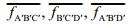
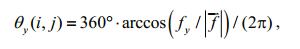
The original image is first converted to a grayscale image. The spatial rectangular coordinate system is set up as shown in Fig. 8, where x-and y-axes represent the positions of the pixels, and the z-axis indicates the gray values of the pixels. For an image G, assuming the position coordinates of the four adjacent pixels A, B, C, and D in the xy-plane are (i+1, j), (i+1, j+1), (i, j+1), (i, j), respectively, and the gray values of these four pixels are I(i+1, j), I(i+1, j+1), I(i, j+1), I(i, j), then the coordinates of the corresponding four points A′, B′, C′, and D′ in 3D space are (i+1, j, I(i+1, j)), (i+1, j+1, I(i+1, j+1)), (i, j+1, I(i, j+1)), (i, j, I(i, j)), respectively. Thus, we can form four planes A′B′C′, A′C′D′, A′B′D′, and B′C′D′ that do not overlap.

|
| Figure 8 Gray surface vector model |
Taking the A′C′D′ plane as an example, the vector
D′C′=(0, 1, I(i, j+1)-I(i, j)), the vector A′D′=(-1, 0, I(i, j)-I(i+1, j)), and the normal vector of the plane A′C′D′ is equal to the vector product of these two vectors: 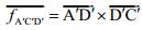
 (20)
(20)This normal vector can be considered as the approximate normal vector of the point D′ in the gray surface A′B′C′D′.
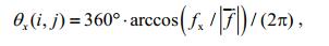
4.2 Gray mapping of the orientation angleWe can further calculate the included angles (orientation angles) of this normal vector and the three coordinate axes as follows:
 (21)
(21) (22)
(22) (23)
(23)where i, j denote the position coordinates of point D in image G; |f| is the norm of f.
The three orientation angles are linearly mapped in the range [0, 255], and the mapping results are used as gray values:
 (24)
(24) (25)
(25) (26)
(26)The mapping of the x-and y-axis orientation angles reflects the change in gray values in the vertical and horizontal orientation, respectively, whereas the mapping of the z-axis orientation angle only reflects the change of the gray values themselves and has no relation with the orientation. Therefore, to highlight the orientation information of the setae, we reconstruct these gray values to obtain the new gray values in the xz-and yz-planes:
 (27)
(27) (28)
(28)According to Eq.24, the above two gray values are linearly stretched to the new gray values Mapxz(i, j) and Mapxz(i, j) to enhance the contrast.
All pixels in image G are processed by the above steps to successively obtain the grayscale images Mapx, Mapy, Mapz, mapxz, mapyz, Mapxz and Mapyz.
4.3 Morphological processingWe first use the 1D Otsu method to binarize Mapxz and Mapyz, and then merge the two resulting binary images into a single image using the logical “and” operation. The median filter is used to remove small noise points from the image. Next, morphological dilation is performed to connect the broken parts of the cell. As described in Section 2.2.1, we extract the big contours and re-apply median filtering to smooth the cellular edges.
Finally, the binary segmentation result can be obtained by morphological erosion and re-extraction of the big contours. We emphasize that the second extraction of big contours is indispensable, because if the noise block is located at the edge of the image, it cannot be removed by the first extraction process.
Figure 9 illustrates the segmentation process for Chaetoceros borealis. To observe the extraction effect of the setae intuitively, the grayscale and color foreground segmentation results are also given as object images in the graph.

|
| Figure 9 Extraction process of Chaetoceros borealis |
We apply the proposed BC algorithm to carry out salient region detection for single-cell and multi-cell non-setae algae microscopic images. Some results are shown in Fig. 10n. In Fig. 10b-m, we compare the results given by 12 recent state-of-the-art saliency measurement methods. These are GS (Wei et al., 2012), IM (Margolin et al., 2013a), LRMR ( Shen and Wu, 2012), SF (Perazzi, 2012), DSR (Li et al., 2013), GC (Cheng et al., 2013), HS (Yan et al., 2013), MC (Jiang et al., 2013), MR (Yang et al., 2013b), PBS (Yang et al., 2013a), PCA (Margolin et al., 2013b) and MS (Tong et al., 2014).

|
| Figure 10 Saliency maps generated by BC algorithm and 12 state-of-the-art methods for non-setae algal cells a. original microscopic images; b. GS; c. IM; d. LRMR; e. SF; f. DSR; g. GC; h. HS; i. MC; j. MR; k. PBS; l. PCA; m. MS; n. BC; o. ground truth. From top to bottom: Prorocentrum sigmoides, Gonyaulax spinifera, Gymnodinium catenatum, Ceratium tripos, Alexandrium tamarense, Prorocentrum minimum, Pleurosigma affine and Akashiwo sanguinea. |
There are various degrees of detection errors in the saliency maps generated by these methods. Some cells have been separated into many isolated fragments by the holes, making it impossible to see the skeleton clearly. In some cellular interiors, the brightness is uneven, and the darker parts are lost in the background. The structure of some cells is missing, and the complete contour cannot be identified. Several detection methods are very sensitive to noise, which causes more background noise in their saliency maps. The effect of some methods is relatively good in that we can see the general morphology of the cells, but the transition zone between the background and foreground is too large to produce significant objects. It is surprising that the saliency map of Prorocentrum minimum generated by the HS method is almost pure white.
Overall, although the number and location of algal cells varies in different pictures, the visual effect of the BC method is always the best, and it accurately locates the cell regions. Salient objects are highlighted and brighter, cleaner and more uniform than in the other methods. This is very close to the ideal ground truth. These phenomena indicate that our method makes full use of the visual perception information in the original images, and we have a reasonable grasp of border-correlation. Note that there are another two “salient” regions caused by impurities in the saliency map of Pleurosigma affine, but these do not affect the subsequent segmentation results.
For non-setae algae, we compared non-interactive GrabCut with seven influential segmentation methods: K-means, Otsu (Otsu, 1979), Canny (Canny, 1986), PCNN (Johnson and Padgett, 1999), Graph Cuts (Boykov and Jolly, 2001), watershed ( Vachier and Meyer, 2005), and LRMR (Shen and Wu, 2012). Some of the binary segmentation results are presented in Fig. 11, where the permutation order of the algae is the same as in Fig. 5.

|
| Figure 11 Binary segmentation results of non-setae algal cells Binary segmentation results of non-setae algal cells |
It is clear that the seven comparative methods exhibit varying degrees of under-or oversegmentation. The K-means method acquires the worst segmentation effect with no separation of cells and background. PCNN even fails for the segmentation of multicellular Prorocentrum minimum. Serious over-segmentation occurs when the Canny and Graph Cuts methods extract those algae containing the cingulum feature (such as Gymnodinium catenatum), preventing cellular boundaries from being obtained. On the contrary, the Otsu and Watershed methods have distinct under-segmentation, which leads to incomplete Ceratium tripos cells. The spire thorn of Prorocentrum sigmoides is entirely lost when segmented by the watershed algorithm. The LRMR method results in protuberant burrs on the object boundary, and loses much of the main body structure of Pleurosigma affine.
In contrast, the objects extracted by our method retain complete biologically morphological details, having elaborate contours and smooth, clear edge that accurately reflect the location, size and shape of the cells. The background noise and edge shadow are both removed. The segmentation effect is particularly good for low contrast algal images, such as Ceratium tripos and Pleurosigma affine.
To inspect the actual effect of the gray surface orientation angle model (GSOAM) algorithm and verify its performance, we conducted an object extraction experiment for a variety of Chaetoceros microscopic images. The performance of GSOAM is compared with various other methodsin Fig. 12.

|
| Figure 12 Binary segmentation results of Chaetoceros cells a. original microscopic images; b. K-means; c. Otsu; d. Canny; e. PCNN; f. Graph Cuts; g. Watershed; h. LRMR; i. GSOAM. From top to bottom: Chaetoceros borealis, Chaetoceros lorenzianus, Chaetoceros diversus, Chaetoceros curvisetus and Chaetoceros densus. |
From the experimental results in Fig. 12, we can see that the segmentation performance of the comparative methods is not stable enough to meet the requirement of extracting setae components from different species of Chaetoceros. The segmentation results generally exhibit four problems: (1) the main body of the cell is broken, and all the setae disappear in the background; (2) a small number of setae with strong background contrast are extracted, but are very short. Many extracted setae are cut off from the middle and divided into two parts, and some setae are even omitted; (3) large regions of noise adhere to the setae parts; (4) the segmentation fails, showing a large black or white region.
On the contrary, our proposed GSOAM method can accurately and effectively separate the cellular structure especially the setae components of different Chaetoceros, and displays better segmentation effects than the other methods. The number of setae is consistent with the original image, and noise interference is removed while key parts are retained.
In addition to the Chaetoceros in Fig. 12, GSOAM was also found to be effective on Chaetoceros compressus, Chaetoceros laciniosus, Chaetoceros atlanticus, Chaetoceros brevis, Chaetoceros pseudocurvisetus, Chaetoceros didymus, and Chaetoceros affinis.
5.2 Quantitative results and evaluationNext, we examine the precision-recall (PR) curves to evaluate the saliency maps of non-setae algae. First, all the saliency values of a saliency map were normalized to [0, 255]. Then we incrementally raised the integer threshold from 0 to 255 to segment this saliency map, and the binary image generated for each threshold was compared with the ground truth to give the precision and recall under the current threshold. The precision (0≤P≤1) and recall (0≤R≤1) were regarded as coordinates, and the PR curve of a single saliency map was obtained through multiple segmentations. The final PR curve was realized by averaging the PR curves of all the saliency maps.
Figure 13 shows the PR curves of the saliency maps generated by the BC method and 23 other saliency detection methods. Besides the 12 methods mentioned above, we also compare the methods of Itti (Itti et al., 1998), GBVS (Harel et al., 2006), SC (Zhai and Shah, 2006), SR (Hou and Zhang, 2007), FT (Achanta et al., 2009), CA (Goferman et al., 2010), MSS (Achanta and Süesstrunk, 2010), BM (Xie and Lu, 2011), CB (Jiang et al., 2011), HC (Cheng et al., 2011) and RC (Cheng et al., 2011). Among these, our method exhibits the highest precision and recall values, and the PR curve is closest to the top right corner point (1, 1). This illustrates that our saliency maps are of higher quality and closer to the ideal effect, and the detected salient regions are very consistent with the actual cell objects. Moreover, by carefully observing all the curves we can further discover a rule: the overall trend of the saliency detection level is constantly improving.

|
| Figure 13 PR Curves Note that the PR curve of the CB method is not actually visible in Fig. 13b. The reason is that the detection results contain some nearly pure black background maps but no salient objects which leads to non-numerical elements emerging in the calculated precision values. As the precision values in the PR curves are the averages of all saliency maps, the curve of this method cannot be drawn. |
Although PR curves are a standard means of evaluation, they have the limitation of only examining the saliency differences between the objects and the background. In addition, we introduce the mean absolute error (MAE) as a metric for evaluation. MAE calculates the average per-pixel difference between a saliency map and its corresponding ground truth. In other words, MAE directly reflects the extent to which the saliency map matches the ground truth, so this measure is complementary to the PR curves. As shown in Fig. 14, our method acquires the lowest MAE score, which means it significantly outperforms the other methods.

|
| Figure 14 Mean absolute error |
For a comprehensive assessment, we further adopted a new weighted F-measure (Margolin et al., 2014) to test the performance of saliency detection. Figure 15 shows the weighted F-measures of various methods. The results indicate that our proposed algorithm performs favorably against the other methods, as it achieves the highest score.

|
| Figure 15 Weighted F-measure |
To quantitatively evaluate the experimental results of each segmentation method for non-setae algae, we plotted a discrete PR graph. As shown in Fig. 16, each binary segmentation image is visually marked on the PR graph. Different markers are used to distinguish the segmentation results given by different methods. By observing the position of each marker, we can see that the distribution of “● (in red)”, corresponding to non-interactive GrabCut, is more concentrated than that of the other types of markers, and is much closer to the point (1, 1). This indicates that our method has greater precision, recall, and higher segmentation quality.

|
| Figure 16 PR Graph |
However, simply emphasizing both high precision and high recall is neither rigorous nor scientific, because there is a mutual inhibition between the precision and recall: if one metric is too high, the other may be weakened. To overcome this contradiction, the F1-measure can be used as a comprehensive evaluation criterion:
 (29)
(29)The higher the F1 value, the more effective the segmentation.
Table 1 lists the F1 values of each method. Our non-interactive GrabCut achieves obviously higher scores than the other methods, and always maintains a relatively high value. This illustrates that our segmentation effect is preferable, and that algal images of different species and complexities can be completely and accurately segmented. Our segmentation performance is more stable and reliable than that of other methods. In addition, the robustness to noise interference is stronger in our segmentation, whereas different degrees of fluctuation occur in the other methods. For example, a minimal value of 0.882 1 appears when the LRMR method segments Pleurosigma affine.

This paper has described the categorical segmentation of cells according to the morphological characteristics of red tide algae in microscopic images.
Regarding non-setae algae, we proposed an automatic segmentation strategy that integrates salient region detection with the GrabCut algorithm.
From the perspective of human visual perception, we designed a novel high-quality salient region detection algorithm for different species of non-setae algae. Our approach simulates the visual attention process of algae experts’ artificial observations. Based on powerful computer vision technology, the proposed framework represents a new direction for the microscopic image analysis of algae or phytoplankton.
The classic GrabCut algorithm requires the user to manually select the rectangular window containing the object or add artificial markers, making it difficult to achieve automatic segmentation. To avoid the tedious human-computer interaction, our method presegments the generated saliency map to obtain cellular position information that can be used for the dual initialization of GrabCut. Moreover, a similarity detection technique has been introduced to exclude pseudo-cellular regions. This non-interactive GrabCut has obvious advantages over the traditional version in terms of stability and accuracy, and extends singleobject segmentation to multi-object segmentation.
In respect of Chaetoceros, we have presented a cell extraction method based on a gray surface orientation angle model. By constructing a gray surface vector model, we achieved the gray mapping of the orientation angles and the reconstruction of the obtained gray values. This allows us to retain the orientation information of the setae and remove prominent noise.
The proposed methods enable the automatic segmentation of algal cells, thus providing the possibility of in -situ and real-time processing of massive microscopic images of red tide algae. This has very important scientific significance and applicability in promoting the development of marine environmental monitoring and HAB early warning systems.
7 ACKNOWLEDGEMENTWe would like to sincerely thank the Key Laboratory of Marine Environment and Ecology of the Ministry of Education at Ocean University, China, and the Research Center for Harmful Algae and Aquatic Environment at Jinan University, China, for offering us the samples and equipment needed to observe and capture the optical micrographs of red tide algae used in this study.
| Achanta R, Hemami S, Estrada F et al. 2009. Frequency-tuned salient region detection. In:Proceedings of IEEE Conference on Computer Vision and Pattern Recognition.IEEE, Miami, FL, USA. p.1 597-1 604. |
| Achanta R, Shaji A, Smith K, et al, 2012. SLIC superpixels compared to state-of-the-art superpixel methods. IEEE Transactions on Pattern Analysis and Machine Intelligence, 34(11): 2 274–2 281. Doi: 10.1109/TPAMI.2012.120 |
| Achanta R, Süesstrunk S. 2010. Saliency detection using maximum symmetric surround. In:Proceedings of the 17th IEEE International Conference on Image Processing.IEEE, Hong Kong, China. p.2 653-2 656. |
| Blaschko M B, Holness G, Mattar M A et al. 2005. Automatic in situ identification of plankton. In:Proceedings of the 7th IEEE Workshops on Applications of Computer Vision.IEEE, Breckenridge, USA. 1:79-86. |
| Boykov Y Y, Jolly M P. 2001. Interactive Graph Cuts for optimal boundary & region segmentation of objects in N-D images. In:Proceedings of the 8th IEEE International Conference on Computer Vision. IEEE, Vancouver, Canada, 1:105-112. https://www.computer.org/csdl/proceedings/iccv/2001/1143/01/114310105-abs.html |
| Canny J, 1986. A computational approach to edge detection. IEEE Transactions on Pattern Analysis and Machine Intelligence, 8(6): 679–698. |
| Cheng M M, Warrell J, Lin W Y et al. 2013. Efficient salient region detection with soft image abstraction. C IEEE International Conference on Computer Vision. IEEE, Sydney, Australia. p.1 529-1 536. |
| Cheng M M, Zhang G X, Mitra N J et al. 2011. Global contrast based salient region detection. In:Proceedings of IEEE Conference on Computer Vision and Pattern Recognition.IEEE, Colorado Springs, USA. p.409-416. |
| Culverhouse P F, Williams R, Benfield M, et al, 2006. Automatic image analysis of plankton:future perspectives. Marine Ecology Progress Series, 312: 297–309. Doi: 10.3354/meps312297 |
| Dimitrovski I, Kocev D, Loskovska S, et al, 2012. Hierarchical classification of diatom images using ensembles of predictive clustering trees. Ecological Informatics, 7(1): 19–29. Doi: 10.1016/j.ecoinf.2011.09.001 |
| Erickson J S, Hashemi N, Sullivan J M, et al, 2012. In situ phytoplankton analysis:there′s plenty of room at the bottom. Analytical Chemistry, 84(2): 839–850. Doi: 10.1021/ac201623k |
| Fischer S, Gilomen K, Bunke H, 2002. Identification of diatoms by grid graph matching. Lecture Notes in Computer Science, 2396: 94–103. Doi: 10.1007/3-540-70659-3 |
| Goferman S, Zelnik-Manor L, Tal A. 2010. Context-aware saliency detection. In:Proceedings of IEEE Conference on Computer Vision and Pattern Recognition. IEEE, San Francisco, USA. p.2 376-2 383. |
| Harel J, Koch C, Perona P. 2006. Graph-based visual saliency.In:Proceedings of Annual Conference on Neural Information Processing Systems. NIPS, Vancouver, Canada. p.545-552. |
| He K M, Sun J, Tang X O, 2010. Guided image filtering. Lecture Notes in Computer Science, 6311: 1–14. Doi: 10.1007/978-3-642-15549-9 |
| Hou X D, Zhang L Q. 2007. Saliency detection:a spectral residual approach. In:Proceedings of IEEE Conference on Computer Vision and Pattern Recognition. IEEE, Minneapolis, USA. p.1-8. |
| Itti L, Koch C, Niebur E, 1998. A model of saliency-based visual attention for rapid scene analysis. IEEE Transactions on Pattern Analysis and Machine Intelligence, 20(11): 1 254–1 259. Doi: 10.1109/34.730558 |
| Jalba A C, Wilkinson M H F, Roerdink J B T M, 2004. Automatic segmentation of diatom images for classification. Microscopy Research and Technique, 65(1-2): 72–85. Doi: 10.1002/(ISSN)1097-0029 |
| Jiang B W, Zhang L H, Lu H C et al. 2013. Saliency detection via absorbing Markov chain. In:Proceedings of IEEE International Conference on Computer Vision. IEEE, Sydney, Australia. p.1 665-1 672. |
| Jiang H Z, Wang J D, Yuan Z J et al. 2011. Automatic salient object segmentation based on context and shape prior. In:Proceedings of British Machine Vision Conference.BMVA Press, Dundee, Britain. p.110.1-110.12. |
| Johnson J L, Padgett M L, 1999. PCNN models and applications. IEEE Transactions on Neural Networks, 10(3): 480–498. Doi: 10.1109/72.761706 |
| Li X H, Lu H C, Zhang L H et al. 2013. Saliency detection via dense and sparse reconstruction. In:Proceedings of IEEE International Conference on Computer Vision. IEEE, Sydney, Australia. p.2 976-2 983. |
| Luo Q Q, Gao Y H, Luo J F, et al, 2011. Automatic identification of diatoms with circular shape using texture analysis. Journal of Software, 6(3): 428–435. |
| Margolin R, Tal A, Zelnik-Manor L. 2013b. What makes a patch distinct? In:Proceedings of IEEE Conference on Computer Vision and Pattern Recognition. IEEE, Portland, USA. p.1 139-1 146. |
| Margolin R, Zelnik-Manor L, Tal A, 2013a. Saliency for image manipulation. The Visual Computer, 29(5): 381–392. Doi: 10.1007/s00371-012-0740-x |
| Margolin R, Zelnik-Manor L, Tal A. 2014. How to evaluate foreground maps? In:Proceedings of IEEE Conference on Computer Vision and Pattern Recognition. IEEE, Columbus, USA. p.248-255. |
| Otsu N, 1979. A threshold selection method from gray-level histograms. IEEE Transactions on Systems, Man, and Cybernetics, 9(1): 62–66. Doi: 10.1109/TSMC.1979.4310076 |
| Perazzi F, Krähenbühl P, Pritch Y et al. 2012. Saliency filters:contrast based filtering for salient region detection. In:Proceedings of IEEE Conference on Computer Vision and Pattern Recognition. IEEE, Providence, USA. p.733-740. |
| Rodenacker K, Hense B, Jüetting U, et al, 2006. Automatic analysis of aqueous specimens for phytoplankton structure recognition and population estimation. Microscopy Research and Technique, 69(9): 708–720. Doi: 10.1002/(ISSN)1097-0029 |
| Rother C, Kolmogorov V, Blake A, 2004. "Grabcut":interactive foreground extraction using iterated Graph Cuts. ACM Transactions on Graphics, 23(3): 309–314. Doi: 10.1145/1015706 |
| Shen X H, Wu Y. 2012. A unified approach to salient object detection via low rank matrix recovery. In:Proceedings of IEEE Conference on Computer Vision and Pattern Recognition. IEEE, Providence, USA. p.853-860. |
| Sosik H M, Olson R J, 2007. Automated taxonomic classification of phytoplankton sampled with imaging-inflow cytometry. Limnology and Oceanography:Methods, 5(6): 204–216. Doi: 10.4319/lom.2007.5.204 |
| Tong N, Lu H C, Zhang L H, et al, 2014. Saliency detection with multi-scale superpixels. IEEE Signal Processing Letters, 21(9): 1 035–1 039. Doi: 10.1109/LSP.2014.2323407 |
| Vachier C, Meyer F, 2005. The viscous watershed transform. Journal of Mathematical Imaging and Vision, 22(2-3): 251–267. Doi: 10.1007/s10851-005-4893-3 |
| Verikas A, Gelzinis A, Bacauskiene M, et al, 2012. Phase congruency-based detection of circular objects applied to analysis of phytoplankton images. Pattern Recognition, 45(4): 1 659–1 670. Doi: 10.1016/j.patcog.2011.10.019 |
| Wei Y C, Wen F, Zhu W J, et al, 2012. Geodesic saliency using background priors. Lecture Notes in Computer Science, 7574: 29–42. Doi: 10.1007/978-3-642-33712-3 |
| Xie Y L, Lu H C. 2011. Visual saliency detection based on bayesian model. In:Proceedings of the 18th IEEE International Conference on Image Processing. IEEE, Brussels, Belgium. p.645-648. |
| Yan Q, Xu L, Shi J P et al. 2013. Hierarchical saliency detection. In:Proceedings of IEEE Conference on Computer Vision and Pattern Recognition. IEEE, Portland, USA. p.1 155-1 162. |
| Yang C, Zhang L H, Lu H C et al. 2013b. Saliency detection via graph-based manifold ranking. In:Proceedings of IEEE Conference on Computer Vision and Pattern Recognition. IEEE, Portland, USA. p.3 166-3 173. |
| Yang C, Zhang L H, Lu H C, 2013a. Graph-regularized saliency detection with convex-hull-based center prior. IEEE Signal Processing Letters, 20(7): 637–640. Doi: 10.1109/LSP.2013.2260737 |
| Zhai Y, Shah M. 2006. Visual attention detection in video sequences using spatiotemporal cues. Annual ACM International Conference on Multimedia, New York, USA. p.815-824. |