 2017, Vol. 35
Institute of Oceanology, Chinese Academy of Sciences
Article Information
- FENG Yongjiu(冯永玖), CHEN Xinjun(陈新军), LIU Yan(刘艳)
- Detection of spatial hot spots and variation for the neon flying squid Ommastrephes bartramii resources in the northwest Pacific Ocean
- Chinese Journal of Oceanology and Limnology, 35(4): 921-935
- http://dx.doi.org/10.1007/s00343-017-6036-2
Article History
- Received Feb. 2, 2016
- accepted in principle Mar. 29, 2016
- accepted for publication May. 25, 2016


2 Key Laboratory of Sustainable Exploitation of Oceanic Fisheries Resources(Shanghai Ocean University), Ministry of Education, Shanghai 201306, China;
3 National Engineering Research Center for Oceanic Fisheries(Shanghai Ocean University), Shanghai 201306, China;
4 Collaborative Innovation Center for Distant-water Fisheries, Shanghai 201306, China;
5 School of Geography, Planning and Environmental Management, University of Queensland, Brisbane Qld 4072, Australia
The neon flying squid (Ommastrephes bartramii) is an important oceanic cephalopod that resides with large stocks over the northwest Pacific Ocean (Chen et al., 2008b; Ichii et al., 2011). The stock of the winter-spring cohort of the squid in this area is a major fishing target for the squid-jigging vessels from Japan, Korea, mainland China and Taiwan (Tian et al., 2009b; Chen et al., 2011). Existing research has addressed various aspects of the O. bartramii in the northwest Pacific Ocean, including the biology and ecology (Ichii et al., 2004; Watanabe et al., 2004; Chen et al., 2008b; Tian et al., 2009a), fisheries resources and stock assessment (Chen and Chiu, 1999; Yatsu et al., 2000; Ichii et al., 2006; Kurosaka et al., 2012), spatiotemporal patterns and their relations with marine environments (Wang et al., 2010; Ichii et al., 2011), fishing ground forecasts (Feng et al., 2014c), and scale effects on spatial patterns (Feng et al., 2016). In particular, the spatiotemporal distribution and its variation for O. bartramii and other pelagic species have been studied for decades (Kulka et al., 1996; Olivar et al., 2003; Bower and Ichii, 2005; Chen et al., 2011), and geographic information systems (GIS) and spatial statistics have increasingly been used as spatial analytical tools to identify the spatiotemporal patterns in fisheries in recent years (Lennert-Cody et al., 2010; Gutiérrez et al., 2011; Cournane et al., 2013).
While scientists have used spatial visualization to graphically illustrate the fishing effort data (Chen et al., 2008a; Wang et al., 2010), there is still a pressing need for experts to discover the spatial patterns and clusters using spatial analysis methods. Geostatistical methods have been used to assess fish abundance (Rivoirard et al., 2000) as well as to design fishery surveys and assess fishery stocks (Petitgas, 2001). Spatial autocorrelation and generalized linear model (GLM) were used to analyze the spatial patterns of the yellowfin tuna (Thunnus albacares) longline catch-per-unit-effort (CPUE) data (Nishida and Chen, 2004). Using an iterative self-organizing data (ISOData) cluster algorithm, Du et al. (2002) investigated the spatiotemporal patterns of fisheries resources from a time series of fisheries data in the East China Sea. Su et al. (2004) explored the spatial heterogeneity and density distribution of demersal fish in the East China Sea through spatial indices such as Geary's C and semi-variograms. While such research has contributed to the understanding of the spatial distribution and patterns of fisheries resources and demonstrated the broad potential of GIS and geostatistical techniques in fisheries research, the spatial distribution of fisheries resources in term of their local spatial aggregation patterns, commonly referred to as spatial hot and cold spots (Morato et al., 2010), are yet to be explored. A hot spot refers to an area (fishing ground) with spatially clustered high values (resource abundance, effort, or catch) while a cold spot typically refers to an area with spatially clustered low values.
With regard to fisheries, several crucial questions can be raised concerning the presence of hot and cold spots across the fishing grounds, the relations between hot/cold spots and the central fishing grounds, and the relations between hot/cold spots and its marine environmental conditions. Analysis of the hot/cold spots of CPUE is an important approach in pelagic fisheries research, which can explore the spatial aggregation of fisheries resources and hence reflect their distribution over space. However, the patterns of hot/cold spots are different with regard to the local autocorrelation statistics (such as Getis-Ord Gi* and Anselin Local Moran's I) and visualization methods used (Chen et al., 2008a; Chun et al., 2013). The hot/cold spot areas can be identified using both the point and polygon-based methods. The point-based assessment is to explore the type of hot/cold spots for each fishing data point while the polygon-based one covering the entire study area is to explore the types of hot/cold spots in neighboring areas of each fishing point. However, disadvantages exist for the polygonbased assessment because it may over-assess the hot or cold spots and include some areas without fishing data points (Feng et al., 2014a; Longley et al., 2015).
This study applies an exploratory spatial data analysis (ESDA) method to detect the spatial patterns and structure of O. bartramii in the northwest Pacific Ocean. Spatial autocorrelation is one ESDA method that measures the degree to which a set of spatial features and their associated data values is clustered (positive spatial autocorrelation) or dispersed (negative spatial autocorrelation) in space (Goodchild, 1986; Getis and Ord, 1992; Anselin, 1995; Koenig, 1999; Getis and Aldstadt, 2010). This method can be implemented to identify and map statistically significant hot and cold spots given a set of weighted features such as CPUE, fishing effort, and catch in fisheries. As a common statistical property of ecological variables observed across geographic spaces, spatial autocorrelation has been widely studied to identify the spatial patterns in ecology (Legendre, 1993), including neotropical migrant songbirds (Lichstein et al., 2002), population density of squirrels in Finland (Koenig and Knops, 1998) and plant ecology (Fortin et al., 1989). Theoretically, there are two levels of indicators to measure spatial autocorrelation (De Smith et al., 2007): 1) global index indicates global pattern of the entire fishery dataset, and 2) local index identifies clusters by evaluating each individual data-point of the study area and maps spatial clusters at local scale.
The purpose of this paper is to analyze both global and local spatial patterns and their variation of O. bartramii in the northwest Pacific Ocean, aiming to improve the understanding of the spatial distributions and dynamics of this squid. The patterns not only include global patterns measured by both summary statistics and global spatial autocorrelation but also include spatial hot and cold spots identified by local spatial autocorrelation statistics. Furthermore, the annual variation of spatial hot and cold spots and the relationship between spatial patterns of the squids and monthly mean sea surface temperature (SST) and monthly mean chlorophyll-a (chl-a) concentration were also analyzed using GIS techniques such as Kriging interpolation, change detection and map comparison. The research outcome improves our understanding of spatiotemporal hotspots and its variation for O. bartramii in the northwest Pacific Ocean and is useful for the sustainable exploitation, assessment, and management of this squid.
2 MATERIAL AND METHOD 2.1 Commercial fishery and environmental dataThe study area is the fishing ground of 150°-160°E and 38°-45°N of O. bartramii in the northwest Pacific Ocean (Fig. 1). Commercial fishery data of O. bartramii over the peak fishing season during July to November from 2007 to 2010 were provided by Chinese Squid-jigging Technology Group (CSCTG). We used 100% of the commercial squid-jigging fishery data for O. bartramii in the areas of 150°-160°E and 38°-45°N, which consisted of 27 fleets from all three fishing corporations (groups) of mainland China including Dalian (6 fleets), Zhoushan (17 fleets) and Ningbo (4 fleets). The fishery raw data include dates of fishing, fishing locations (longitude and latitude), the number of fishing vessels operated per day, and daily catch of vessels. Some vessels recorded and reported their daily catch with fishing locations and times, while other vessels only reported the total daily catch with a large spatial grid. To eliminate the influence of the spatio-temperal difference of the vessels, the fishery data were aggregated annually and tessellated to a spatial scale of 0.5°×0.5°, in the form of CPUE (Tian et al., 2009b; Chen et al., 2011). The nominal CPUE was calculated as:
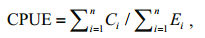 (1)
(1)where n is the total number of fishing records within an area of 0.5°×0.5°, Ci is the catch (in tones, t) of a fishing vessel per record and E is the corresponding fishing effort, i.e., number of fishing operations.

|
| Figure 1 The study area and the dataset used |
Each data point in Fig. 1 contains the averaged CPUE values over the July to November period in each year. As such, the focus of this research is the annual variation in spatial patterns rather than the seasonal changes. At the 0.5°×0.5° spatial scale, there are 86 data points in 2007, 109 in 2008, 100 in 2009, and 165 in 2010 in the study area. Additionally, to examine the interaction between hot/cold spots and the ocean environmental conditions, monthly SST and chl-a data corresponding to each CPUE data point were extracted for the years during 2007-2010. These oceanographic data, SST and chl-a with a spatial resolution of 4km, were collected from OceanColor Web of NASA (IOCCG, http://oceancolor.gsfc.nasa.gov).
2.2 Spatial autocorrelation 2.2.1 Global spatial autocorrelationGlobal spatial autocorrelation was employed to detect the potential global spatial patterns of O. bartramii in the northwest Pacific Ocean. This is measured using the Moran's I index (Sokal and Oden, 1978; Goodchild, 1986) as:
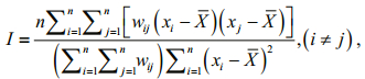 (2)
(2)where n is the number of samples (data points of the fishery resources); xi and xj are the properties (i.e. CPUE values) of sample i and j, respectively; X is the averaged value of all samples; and wij is the spatial weight matrix indicating the spatial adjacency relation between samples i and j. Generally, the spatial weight matrix wij is defined using either an adjacency standard or a distance standard (Getis and Aldstadt, 2010). In this paper, an inverse distance method was utilized to define the spatial weight matrix of the point-based fishing data.
The value of Moran's I ranges from -1 to 1. A value of Moran's I larger than 0 indicates a positive correlation (i.e., CPUE tends to be clustered), whereas a value smaller than 0 indicates a negative correlation (i.e., CPUE tends to be dispersed). A value of 0 for Moran's I indicates no autocorrelation, that is, a random distribution of fisheries resources.
Two additional measures, z-score and P-avalue, are usually computed with the Moran's I index to indicate whether or not a null hypothesis that states the CPUE are randomly distributed across the study area should be rejected. The z-score is a statistical test to determine whether the null hypothesis of no spatial autocorrelation should be rejected and the P-avalue gives the probability of obtaining the results at least as extreme as those observed, if the null hypothesis is true (Mitchell, 2005). A very small P-avalue (P < 0.05) is associated with a very high or low z-score (>1.96 or < -1.96), meaning that there is less than 5% probability that the observed spatial pattern is the result of a random process; in other words, the null hypothesis of no spatial autocorrelation can be rejected at the 95% confidence level.
2.2.2 Local spatial autocorrelationAlthough Moran's I can be used to describe the patterns in the global distribution of all data for O. bartramii, it does not describe the pattern at the local level (Longley et al., 2005), i.e. whether there are spatial clusters for this species. Therefore, local spatial autocorrelation statistics are needed to assess the dependency relationships across space at a local scale (Getis and Ord, 1992; Anselin, 2005; Peeters et al., 2015). The local spatial autocorrelation can be measured using Getis-Ord Gi* statistic, which is given as:
 (3)
(3)where S is the standard deviation of all data points in term of CPUE, other elements in this equation bear the same meaning as in Eq.2. Similar to that of the Moran's I index, Getis-Ord Gi* statistic also generate two additional measures, the z-score for each sample and a P-avalue.
Statistically, a z-score larger than 2.58 (P < 0.01) indicates a hot spot while a z-score lower than -2.58 (P < 0.01) indicates a cold spot. A hot spot reflects that CPUE points with high values are surrounded by other CPUE points with similarly high values; in contrast, a cold spot reflects that CPUE points with low values are surrounded by other CPUE points with similarly low values. On the other hand, the hot spots also indicate the areas with clustered high catch while the cold spots indicate the areas with clustered low catch.
If a z-score is between -2.58 and -1.96 or between 1.96 and 2.58, then the corresponding P-avalue will be between 0.01 and 0.05. As a result, the underlying pattern could be a hot or cold spot at the 0.05 significance level, but the null hypothesis cannot be rejected at the 0.01 significance level, and the pattern could also be the result of randomly distributed CPUE. If a z-score is between -1.96 and -1.65 or between 1.65 and 1.96, the corresponding P-avalue will be between 0.05 and 0.10. Such a value indicates that support for the distribution being a hot or cold spot is weaker and the hypothesis that it is not the result of a random process cannot be accepted at the 0.05 significance level. Moreover, a z-score between -1.65 and 1.65 is considered being not statistically significant.
2.3 Comparison methods for hot/cold spotsA GIS overlay analysis based on two shape-format maps (Mitchell, 2005) was used to analyze the annual variation of location and spatial boundary of hot and cold spots. Such overlay analysis derives additional information from two or more layers covering the same area and then produces a comparison map (Longley et al., 2015). In this paper, the overlay method was utilized to detect the spatiotemporal differences between two adjacent years from 2007 to 2010, and consequently, to identify and visualize the persistence and variation of hot and cold spots. The comparison map focuses on four categories including 1) areas of persistent hot spots, 2) areas with changed states from a hot spot to a cold spot, 3) areas with changed states from a cold spot to a hot spot, and 4) areas of persistent cold spots. Both the persistence and change of the other categories with z-scores ranging from -2.58 to 2.58 were not considered in this research.
A change matrix was used to retrieve the percentages of hot and cold spots in term of area size (Pontius et al., 2004; Aldwaik and Pontius Jr, 2012), hence to analyze the annual variation of area size. The change matrix is a specific table layout, commonly generated by a cell-by-cell comparison (Pontius et al., 2004; Aldwaik and Pontius Jr, 2012), that allows assessing the changes between two rasterized maps. Each row of the matrix represents the classes of an earlier map, while each column represents the classes of a later map.
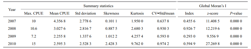
3 RESULT 3.1 Summary statistics and global patternsThe spatial patterns of O. bartramii were detected using both summary statistics and the global Moran's I index (Table 1), and the frequency distributions of the data for the four years are charted in Fig. 2.
|

|
| Figure 2 The histograms and actual distributions of CPUE for O. bartramii in the northwest Pacific Ocean |
Table 1 shows, of the four years, both the maximum CPUE (7.2) and mean CPUE (2.255 8) in 2009 are the smallest, indicating the lowest catch (8 878 t) for O. bartramii. The mean CPUE of the other years are larger and their catches are 29 872 t, 26 906 t and 15 862 t in 2007, 2008 and 2010, successively. Although the skewness values are all positive, the value of 2007 is only 0.101 1, suggesting a very weak left-skew and the tails are almost equally long at both the left and right sides (also see Fig. 2). For the other three years, the left-skew are stronger with much larger skewness, indicating that the left tails are shorter and the mass of the distributions is concentrated on the left of the figures (Fig. 2). The kurtosis values smaller than 3 in 2007 and 2008 indicate platykurtic distributions, whereas the values larger than 3 in 2009 and 2010 indicate leptokurtic distributions (also see Fig. 2). The coefficients of variation (CV) of 2007 and 2009 are both smaller, which indicate lower variations of O. bartramii across space while those of 2008 and 2010 are larger which indicate higher variations of this squid across space.
The positive value of Moran's I index (c.f. Table 1) indicates that the spatial distribution of the O. bartramii resources exhibits a degree of clustering each year. However, clustering characteristics of 2009 are not strong as those of the other years because the Moran's I index is only 0.293 0, but the P-avalue still indicates that a random spatial distribution can be rejected at the 0.01 significance level. On the other hand, the high z-scores (with P < 0.01) for Moran's I also revealed significantly clustered distributions of O. bartramii.
3.2 Hot and cold spotsThe hot and cold spots of O. bartramii were detected by using Getis-Ord Gi* based on the CPUE data shown in Fig. 1. The computation of Getis-Ord Gi* was conducted in ArcGIS 10.1 and it returned both z-score and P-avalue for each CPUE point. The z-scores were categorized depending on Eq.3 and the maps of the hot and cold spots were produced from 2007 to 2010 (Fig. 3). The polygon-based z-score maps in Fig. 3 are the result of Kriging interpolation using the point-based rendering z-scores. As a result, the interpolated z-score values, where there are no CPUE points, could not have high accuracies. However, the focus of this paper is the hot and cold spots that supported by sufficient data points and these spots were not affected by the spatial interpolation (Fig. 3). Of all hot and cold spots, the cold spot of 2009 had the smallest area and has been supported by the least number of data points; as a consequence, it was relatively less reliable compared with the others.

|
| Figure 3 Statistically significant (P-value=0.01) hot and cold spots for O. bartramii in the northwest Pacific Ocean from 2007 to 2010 |
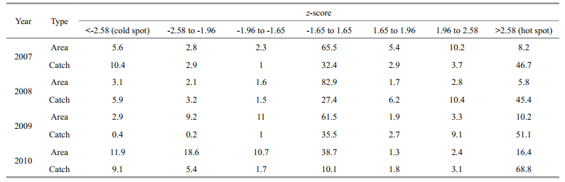
The percentages of hot/cold spots (see Table 2) for all four years were calculated using the polygonbased z-score (includes 7 types of statistics) shown in the maps of Getis-Ord Gi* indexes (Fig. 3).
|
Table 2 shows, the hot spots occupied 8.2% in 2007 and 5.8% in 2008 of the study area while the percentage increased to 10.2% in 2009 and 16.4% in 2010. The areas of cold spots were 5.6%, 3.1% and 2.9% of the study area in 2007, 2008 and 2009, respectively, while this percentage drastically increased to 11.9% in 2010. This change indicates that the areas with "low CPUE values surrounded by similar low CPUE values" have drastically increased in 2010. The areas with significance larger than 0.01 (s.g.>0.01) were 91.1% of the study area in 2008. Although the percentages were smaller, they also reached 86.2%, 86.9% and 71.7% in 2007, 2009 and 2010, respectively, demonstrating that most of the study area was neither hot nor cold spots. Table 2 also shows that almost half of the squids from 2007 to 2009 reported by Chinese mainland squid-jigging fleets were caught in hot spots while this percentage reached its peak at 68.8% in 2010. The percentage of the catch in the sea area being not statistically significant (-1.65 < z-score < 1.65) ranks the second each year, mainly attributed to its dominated percentage in area size. In addition, the percentage of catch in cold spots is much lower but it is not the lowest one each year.
Moreover, location and CPUE distribution of each hot and cold spot was consequently detected and analyzed in detail. Table 3 shows the boundaries and summary statistics of the hot/cold spots, including counts, minimum, maximum and mean CPUE, and standard deviations.
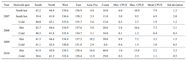
There were 2 hot and 1 cold spots in 2007 while only 1 hot and 1 cold spots in each year during 2008-2010 for O. bartramii in the northwest Pacific Ocean (Fig. 3 and Table 3).
The hot spots in 2007 were located at north and south of the study area, respectively, and the north one includes 10 data points and has a mean CPUE of 7.9 occupying 4.9% of the study area; in contrast, the south one has a mean CPUE of 6.9 and occupied 3.3%. In addition, the cold spot in 2007 consisting of 13 data points and occupying 5.6% of the study area, and its mean CPUE (1.9) is much lower than those of the hot spots (Table 3).
The hot spot in 2008 was spatially close to the north one in 2007, but the area (with 5.8%, see Table 2) of the former is slightly bigger. Table 3 shows the hot spot in 2008 includes 20 data points and its mean CPUE is 7.3, while the cold spot including 10 data points and occupying 3.1% of the study area only has a mean CPUE of 0.4, which is the lowest of the four years during 2007-2010.
The hot spot in 2009 includes 30 data points and occupied 10.2% of the study area, having a mean CPUE of 3.3 that is much lower than those of 2007 and 2009. Meanwhile, the cold spot in 2009 only includes 4 data points and occupied 2.9% of the study area, having a mean CPUE of 1.0 that is smaller than those of 2007 and 2010 but larger than that of 2008.
In addition, the hot spot in 2010 was spatially close to the north hot spot in 2007 and those of 2008 and 2009. This hot spot includes 46 data points and has a mean CPUE of 5.2, and its area (occupied 16.4%) is bigger than those of the other three years. In addition, the mean CPUE of the cold spot is 1.1, which is smaller than that of 2007 but bigger than those of 2008 and 2009. The cold spot includes 29 data points and occupied 11.9% of the study area, much bigger than the cold spots of the other three years.
3.3 Annual variation of hot and cold spots 3.3.1 Annual variation of the boundaryThree change maps of hot and cold spots were generated for comparisons between 2007 and 2008, 2008 and 2009, and 2009 and 2010 (Fig. 4). Only two categories, i.e. persistent hot spots and persistent cold spots, have been identified from the comparison maps. Other categories of variation related to areas being not statistically significant were not considered in this research, in that these areas usually were not central fishing grounds across space and time. These categories include the persistence of areas being not statistically significant (z-scores ranging from -2.58 to 2.58), the change between areas being not statistically significant, and the change between hot/ cold spots and areas being not statistically significant. The comparison between 2007 and 2008 (Fig. 4a) shows that there were 1 cold spot (centered at 154°E/40.5°N) with state unchanged and 1 hot spot (centered at 156°E/44°N) with state unchanged. Meanwhile, only 1 hot spot with state unchanged was identified for each comparison from 2008 to 2010, i.e. 2008 vs 2009 and 2009 vs 2010, and these unchanged hot spots were centered at 155.8°E/43.5°N and centered at 155.8°E/43°N, respectively. Most importantly, the area centered at 156°E/43.5°N was a persistent hot spot during 2007 to 2010, indicating a crucial central fishing ground for O. bartramii in the study area. Moreover, change or variation between areas being not statistically significant, the "Other" category in Fig. 4, has dominated the study area.

|
| Figure 4 Annual variation of boundary for hot and cold spots of O. bartramii in the northwest Pacific Ocean from 2007 to 2010 |
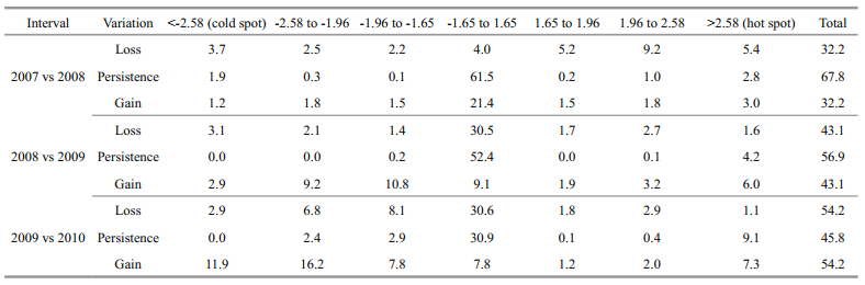
Using a cell-by-cell comparison derived change matrix, annual variation of hot and cold spots of O. bartramii in term of area size was assessed between two adjacent years from 2007 to 2010 (Table 4). The persistence indicates the agreement between two adjacent years, and the loss is equal to the gain between two adjacent years as the total area under study is constant.
|
Table 4 shows 67.8% of the study area remained unchanged from 2007 to 2008. The areas identified as hot spots in 2007 shrunk from 8.2% to 2.8% in 2008 (a loss of 5.4%, c.f. Table 4) but there was a 3.0% gain in other areas resulting in a total hot spot coverage in 2008 of 5.8% (c.f. Table 2). Meanwhile, the areas identified as cold spots in 2007 shrunk from 5.6% to 1.9% in 2008 (a loss of 3.7%, c.f. Table 4) but there was a 1.2% gain in other areas resulting in a total cold spot coverage in 2008 of 3.1% (c.f. Table 2). This also means both the hot and cold spots suffered losses of coverage from 2007 to 2008, but the area identified as being not statistically significant in 2007 expanded from 65.5% to 82.9% in 2008 (c.f. Table 2).
Similarly, Table 4 shows 56.9% of the study area remained unchanged from 2008 to 2009, which is mainly attributed to the area (52.4%) identified as being not statistically significant. The areas identified as hot spots in 2008 shrunk from 5.8% to 4.2% in 2009 (a loss of 1.6%, c.f. Table 4) but gained 6.0% in other areas resulting in a total hot spot coverage in 2009 of 10.2% (c.f. Table 2). Meanwhile, the areas identified as cold spots in 2008 totally disappeared in 2009 at the same location (a loss of 3.1%, c.f. Table 4) but gained 2.9% in other areas resulting in a total cold spot coverage in 2009 of 2.9% (c.f. Table 2). This means coverage of hot spots significantly expanded from 2008 to 2009, but the coverage of cold spots slightly decreased and completely shifted its location (c.f. Fig. 3).
In addition, Table 4 shows 45.8% of the study area remained unchanged from 2009 to 2010, which is mainly attributed to 30.9% persistence of the area identified as being not statistically significant. The areas identified as hot spots in 2009 slightly shrunk from 10.2% to 9.1% in 2010 (a loss of 1.1%, c.f. Table 4) but there was a 7.3% gain in other areas resulting in a total hot spot coverage in 2010 of 16.4% (c.f. Table 2). Meanwhile, the areas identified as cold spots in 2009 totally disappeared in 2010 at the same location (a loss of 2.9%, c.f. Table 4) but gained 11.9% in other areas resulting in a total cold spot coverage in 2010 of 11.9% (c.f. Table 2). This means the coverage of both hot and cold spots significantly increased from 2009 to 2010, but the cold spot completely shifted its location (c.f. Fig. 3).
4 DISCUSSION 4.1 Factors affecting the hot and cold spotsIdentified hot and cold spots, to some degree, were affected by several factors such as the monthly variation of O. bartramii, the spatial distribution of the fishing data, and the selection of the z-score and P-avalue.
It is natural that the monthly variation has impacts on the results as the nominal CPUE was computed based on five months across July-November from 2007 to 2010. By using central feature tool (Mitchell, 2005) in ArcGIS 10.1, the centroid of fishing ground was computed for each month from July to November. These centroids show that their locations were geographically close to each other for different months of the same year. As a result, despite the monthly variation of the spatial distribution of O. bartramii, the influence of such variations on the results was very limited (Chen et al., 2012).
The spatial distribution of commercial fishery data (include CPUE and fishing effort) substantially affects the results of hot and cold spots. In fact, statistically significant hot and cold spots are the result of comparison between different sub-areas of the same study area. Evidently, hot spots substantially are central fishing grounds because a great majority of the catches reported being from these areas (c.f. Table 2). Moreover, Table 3 shows the hot and cold spots were related to different fishing sea areas with unique locations and CPUE features characterized by the summary statistics. These statistics indicate that fishing areas with high catches would likely result in hot spots while low catches would likely result in cold spots. Overall, the variation in spatial hot and cold spots of fisheries resources is a reflection of the variation of central fishing grounds (Feng et al., 2014a, b).
The hot and cold spots were also affected by the selection of the z-score (P-avalue) that is a benchmark for the definition of the spots. In this research, a z-score larger than 2.58 or smaller than -2.58 was adopted to define the hot or cold spots, which correspond to a high probability (99%) of rejecting the null hypothesis. A z-score value of -1.96 or 1.96 corresponding to a 95% confidence level (P-value=0.05) has also been applied to define the hot or cold spots (Mitchell, 2005; Feng et al., 2014a). Compared to the 0.01 P-avalue scheme, the areas of hot and cold spots under 0.05 P-value will increase substantially. As a consequence, those spots under 0.05 P-avalue cannot be supported by sufficient fishing points, resulting in lower reliability in analysis of spatial patterns, therefore this research used the 0.01 P-avalue instead of 0.05 P-value.
Annual variation analysis shows only the persistent hot spots and the persistent cold spots were observed from 2007 to 2010, while no areas changed from a cold spot to a hot spot or from a hot spot to a cold spot were identified during the same period (c.f. Fig. 4). This means it is unlikely that areas shift their states between hot and cold spots. The areas being not statistically significant and not supported by sufficient fishing points in a year can change its state to be hot spots in the next year (see the gains of the hot spots in Table 4), indicating a new central fishing area was formed. The cold spots also gained areas from those being not statistically significant in a previous year, indicating the decrease of CPUE (perhaps the resources) that maybe affected by the oceanic environments.
4.2 Influence of ocean environments on hot/cold spotsPrevious research shows that the pelagic fish population (e.g. O. bartramii) has a migratory behavior and is vertically migrating day and night (Chen et al., 2011), which may be caused by a change in the marine environments the species inhabit. Several marine environmental factors have been identified as the main reasons for the variation of central fishing grounds, which include the cold Oyashio and warm Kuroshio Currents, SST, chl-a concentration, and global climate change (Chen et al., 2008a; Wang et al., 2010; Ichii et al., 2011). To analyze the influence of ocean environments on hot and cold spots, two important factors, monthly mean SST and monthly mean chl-a concentrations, were selected and processed to be contour lines (Figs. 5, 6) in ArcGIS 10.1.

|
| Figure 5 The relationship between monthly mean SST and hot (in red color) and cold (in blue color) spots clusters in the northwest Pacific Ocean from 2007 to 2010 |

|
| Figure 6 The relationship between monthly mean chl -a concentrations and hot (in red color) and cold (in blue color) spots clusters in the northwest Pacific Ocean from 2007 to 2010 |
The Kuroshio is a warm ocean current where the SST is higher than 15℃ while the Oyashio is a cold ocean current where the SST is lower than 5℃ (Chen et al., 2012). These two currents have a major effect on the spatial distribution of O. bartramii in the northwest Pacific Ocean (Chen et al., 2011; Feng et al., 2014b). Figure 5 shows the monthly mean SST was the highest in August for all four years and it decreased gradually from September to November. In addition, warm water masses were identified in October and November 2008, November 2009, and October 2010. For 2007, the north hot spot was formed mainly by the high catches in August and September where the mean SST was around 15℃ on the north side of warm Kuroshio Current; whereas, the south hot spot was formed mainly by the high catch in July where the mean SST was in the range of 15-18℃ on the south side of warm Kuroshio Current. Meanwhile, the cold spot this year was formed mainly by the low catch in July, August, and November, where the mean SST were much higher than warm Kuroshio Current.
The hot spot in 2008 was formed mainly by the high catches in July, August and September where the mean SST was around 15℃ in relation to warm Kuroshio Current; whereas, the cold spot this year was formed mainly by the low catches also in August and September in other areas where the mean SST were much higher. Figure 5 also shows that the hot spot in 2009 was formed mainly by the high catches in July, August and October where the mean SST was around 15℃ between warm Kuroshio Current and cold Oyashio Current; however, the cold spot formed by only few data points with low CPUE cannot be attributed to SST. The hot spot in 2010 was formed mainly by the high catches in all months except October; whereas, the cold spot was formed mainly by the low catch in all months in other areas where the mean SST was much higher.
Figure 5 also shows that the cold Oyashio Currents were weak in the northwest Pacific Ocean from 2007 to 2010 which only affected a small part of the study area. As a consequence, the warm Kuroshio Current has dominated in the northwest Pacific Ocean, resulting in a good harvest in most of the traditional fishing grounds in 2007 (Chen et al., 2011, 2012; Feng et al., 2014b). Compared with 2007, CPUE in 2008 was higher near 157°E/44°N but it was much lower near 157°E/40°N. The warm Kuroshio Current in 2010 was relatively weak and the cold Oyashio Current was relatively strong, and the fishing grounds in the best fishing seasons moved with the cold Oyashio Current. The hot and cold spots map of 2010 shows that the hot spot is located to the north of 42°N while the cold spot is located to the south of 42°N. The spatial patterns identified by the spatial autocorrelation is very consistent with the fishing grounds of the study area, which reveals the clustering distributions of O. bartramii as well as the locations of the central fishing grounds.
In addition to SST, chl-a concentration is another important factor affecting the spatial patterns of O. bartramii in the northwest Pacific Ocean. Generally, the chl-a concentration at higher latitudes are higher than those at lower latitudes (Chen et al., 2011) and literature shows that there is a biomass front in the northwest Pacific Ocean, i.e. the transition zone chlorophyll front (TZCF) (Ichii et al., 2011). The TZCF is the boundary between the subtropical regions with low chl-a concentrations and the subarctic regions with high chl-a concentrations (Polovina et al., 2001). It was acknowledged that the chl-a concentration within the TZCF is about 0.2 mg/m3 and O. bartramii commonly forages within the sea at the north of the TZCF (Chen et al., 2011). Figure 6 shows the overlay maps of monthly mean chl-a concentrations and hot and cold spot patterns of O. bartramii.
Figure 6 indicates that the TZCFs during July to August show a trend of moving north while the TZCFs during September to November show a trend of moving south. These findings essentially accord with those reported by other scientists (Chen et al., 2011; Ichii et al., 2011). Figure 6 also demonstrates that the chl-a concentration was higher than 0.3 mg/m3 in the north hot spot of 2007 while it was also higher than 0.3 mg/m3 in the south hot spot except in September and November. In contrast, the concentration in the cold spot was lower than 0.3 mg/m3 except in August and October 2007. The chl-a concentration in the hot spot in 2008 was higher than 0.3 mg/m3 except in July, while it was lower than 0.3 mg/m3 in the cold spot except in August and October (the same months as 2007).
The chl-a concentration in 2009 was all higher than 0.3 mg/m3 in both hot and cold spots. This might be because the cold spot this year only formed by few data points with low CPUE and which also cannot be attributed to the chl-a. The chl-a concentration in 2010 was higher than 0.3 mg/m3 in the hot spot while it was lower than 0.3 mg/m3 in the cold spot except in October and November.
Research conducted by Chen et al. (2011) showed that the central fishing grounds in the northwest Pacific Ocean are mainly distributed within areas with a chl-a concentration in the range of 0.2-0.8 mg/m3. Specifically, this research shows the chl-a concentration is above 0.3 mg/m3 in hot spots while it is smaller than 0.3 mg/m3 in cold spots except for the specific months above-mentioned. From a perspective of spatial autocorrelation, both the hot and cold spots are strongly spatially clustered and a high frequency of fishing activity was reported in such areas, whereas the other areas showing random or non-clustered distributions are not spatially clustered. However, only the hot spots, where both the CPUE and the percentages of catches and are usually high, can be considered as central fishing grounds.
5 CONCLUSIONThis paper carried out an exploratory spatial data analysis of O. bartramii in the northwest Pacific Ocean from 2007 to 2010, using summary statistics and spatial autocorrelations. The hot and cold spots configurations have been explored and then visually mapped in a GIS environment. We concluded that the hot spots, where both the CPUE and the percentages of catches are usually high, are central fishing grounds, and both the hot and cold spots are affected by the ocean environments such as SST and chl-a. While the results described here are based on an analysis of the fishery data at the spatial scale of 0.5°×0.5°, additional work is required to investigate the sensitivity of these results and to explore the spatial patterns in fishery data more generally at the spatial scale used.
| Aldwaik S Z, Pontius Jr R G, 2012. Intensity analysis to unify measurements of size and stationarity of land changes by interval, category, and transition. Landscape and Urban Planning, 106(1): 103–114. Doi: 10.1016/j.landurbplan.2012.02.010 |
| Anselin L, 1995. Local indicators of spatial association-LISA. Geographical Analysis, 27(2): 93–115. |
| Anselin L. 2005. Exploring Spatial Data with GeoDaTM: A Workbook. Spatial Analysis Laboratory, Department of Geography, University of Illinois at Urbana-Champaign, Urbana, IL. |
| Bower J R, Ichii T, 2005. The red flying squid (Ommastrephes bartramii):A review of recent research and the fishery in Japan. Fisheries Research, 76(1): 39–55. Doi: 10.1016/j.fishres.2005.05.009 |
| Chen C S, Chiu T S, 1999. Abundance and spatial variation of Ommastrephes bartramii (Mollusca:Cephalopoda) in the eastern North Pacific observed from an exploratory survey. Acta Zoologica Taiwanica, 10(2): 135–144. |
| Chen X J, Cao J, Chen Y, Liu B L, Tian S Q, 2012. Effect of the Kuroshio on the spatial distribution of the red flying squid Ommastrephes Bartramii in the Northwest Pacific Ocean. Bulletin of Marine Science, 88(1): 63–71. Doi: 10.5343/bms.2010.1098 |
| Chen X J, Chen Y, Tian S Q, Liu B L, Qian W G, 2008a. An assessment of the west winter-spring cohort of neon flying squid (Ommastrephes bartramii) in the northwest Pacific Ocean. Fisheries Research, 92(2-3): 221–230. Doi: 10.1016/j.fishres.2008.01.011 |
| Chen X J, Liu B L, Chen Y, 2008b. A review of the development of Chinese distant-water squid jigging fisheries. Fisheries Research, 89(3): 211–221. Doi: 10.1016/j.fishres.2007.10.012 |
| Chen X J, Tian S Q, Chen Y, Cao J, Ma J, 2011. Fishery Biology for Ommastrephes bartramii in the Northwestern Pacific Ocean. Science Press, Beijing. |
| Chun Y W, Griffith D A, 2013. Spatial Statistics and Geostatistics:Theory and Applications for Geographic Information Science and Technology. SAGE, London. |
| Cournane J M, Kritzer J P, Correia S J, 2013. Spatial and temporal patterns of anadromous alosine bycatch in the US Atlantic herring fishery. Fisheries Research, 141: 88–94. Doi: 10.1016/j.fishres.2012.08.001 |
| de Smith M J, Goodchild M F, Longley P, 2007. Geospatial ANALYSIS:A Comprehensive Guide to Principles, Techniques and Software Tools. Troubador Publishing Ltd, Leicester, UK. |
| Du Y Y, Zhou C H, Shao Q Q, Su F Z, 2002. Extracting spatiotemporal patterns from ocean fishery dataset in East China Sea using spatial cluster. High Technology Letters, 12(1): 91–95. |
| Feng Y J, Chen X J, Liu Y, 2016. The effects of changing spatial scales on spatial patterns of CPUE for Ommastrephes bartramii in the northwest Pacific Ocean. Fisheries Research, 183: 1–12. Doi: 10.1016/j.fishres.2016.05.006 |
| Feng Y J, Chen X J, Yang M X, Huo D, Zhu G P, 2014b. An exploratory spatial data analysis-based investigation of the hot spots and variability of Ommastrephes bartramii fishery resources in the northwestern Pacific Ocean. Acta Ecologica Sinica, 34(7): 1841–1850. |
| Feng Y J, Chen X J, Yang X M, Gao F, 2014c. HSI modeling and intelligent optimization for fishing ground forecasts using a genetic algorithm. Acta Ecologica Sinica, 34(15): 4333–4346. |
| Feng Y J, Yang M X, Chen X J, 2014a. Analyzing spatial aggregation of Ommastrephes bartramii in the Northwest Pacific Ocean based on Voronoi diagram and spatial autocorrelation. Acta Oceanologica Sinica, 36(12): 74–84. |
| Fortin M J, Drapeau P, Legendre P, 1989. Spatial autocorrelation and sampling design in plant ecology. Vegetatio, 83(1-2): 209–222. Doi: 10.1007/BF00031693 |
| Getis A, Aldstadt J. 2010. Constructing the spatial weights matrix using a local statistic. In: Anselin L, Rey S J eds. Perspectives on Spatial Data Analysis. Springer, Berlin Heidelberg. p. 147-163. |
| Getis A, Ord J K, 1992. The analysis of spatial association by use of distance statistics. Geographical Analysis, 24(3): 189–206. |
| Goodchild M F, 1986. Spatial Autocorrelation. Geo Books, Norwich. |
| Gutiérrez N L, Masello A, Uscudun G, Defeo O, 2011. Spatial distribution patterns in biomass and population structure of the deep sea red crab Chaceon notialis in the Southwestern Atlantic Ocean. Fisheries research, 110(1): 59–66. Doi: 10.1016/j.fishres.2011.03.012 |
| Ichii T, Mahapatra K, Okamura H, Okada Y, 2006. Stock assessment of the autumn cohort of neon flying squid(Ommastrephes bartramii) in the North Pacific based on past large-scale high seas driftnet fishery data. Fisheries Research, 78(2-3): 286–297. Doi: 10.1016/j.fishres.2006.01.003 |
| Ichii T, Mahapatra K, Sakai M, Inagake D, Okada Y, 2004. Differing body size between the autumn and the winter-spring cohorts of neon flying squid (Ommastrephes bartramii) related to the oceanographic regime in the North Pacific:a hypothesis. Fisheries Oceanography, 13(5): 295–309. Doi: 10.1111/fog.2004.13.issue-5 |
| Ichii T, Mahapatra K, Sakai M, Wakabayashi T, Okamura H, Igarashi H, Inagake D, Okada Y, 2011. Changes in abundance of the neon flying squid Ommastrephes bartramii in relation to climate change in the central North Pacific Ocean. Marine Ecology Progress Series, 441: 151–164. Doi: 10.3354/meps09365 |
| Koenig W D, Knops J M H, 1998. Testing for spatial autocorrelation in ecological studies. Ecography, 21(4): 423–429. Doi: 10.1111/eco.1998.21.issue-4 |
| Koenig W D, 1999. Spatial autocorrelation of ecological phenomena. Trends in Ecology & Evolution, 14(1): 22–26. |
| Kulka D W, Pinhorn A T, Halliday R G, Pitcher D, Stansbury D, 1996. Accounting for changes in spatial distribution of groundfish when estimating abundance from commercial fishing data. Fisheries research, 28(3): 321–342. Doi: 10.1016/0165-7836(96)00508-5 |
| Kurosaka K, Yamashita H, Ogawa M, Inada H, Arimoto T, 2012. Tentacle-breakage mechanism for the neon flying squid Ommastrephes bartramii during the jigging capture process. Fisheries Research, 121-122: 9–16. Doi: 10.1016/j.fishres.2011.12.016 |
| Legendre P, 1993. Spatial autocorrelation:trouble or new paradigm?. Ecology, 74(6): 1659–1673. Doi: 10.2307/1939924 |
| Lennert-Cody C E, Minami M, Tomlinson P K, Maunder M N, 2010. Exploratory analysis of spatial-temporal patterns in length-frequency data:an example of distributional regression trees. Fisheries Research, 102(3): 323–326. Doi: 10.1016/j.fishres.2009.11.014 |
| Lichstein J W, Simons T R, Shriner S A, Franzreb K E, 2002. Spatial autocorrelation and autoregressive models in ecology. Ecological Monographs, 72(3): 445–463. Doi: 10.1890/0012-9615(2002)072[0445:SAAAMI]2.0.CO;2 |
| Longley P A, Goodchild M F, Maguire D J, Rhind D W, 2015. Geographic Information Science and Systems. John Wiley & Sons, London. |
| Mitchell A, 2005. The ESRI guide to GIS analysis, Volume 2:Spatial Measurements and Statistics. Esri Press, Redlands. |
| Morato T, Hoyle S D, Allain V, Nicol S J, 2010. Seamounts are hotspots of pelagic biodiversity in the open ocean. Proceedings of the National Academy of Sciences of the United States of America, 107(21): 9707–9711. Doi: 10.1073/pnas.0910290107 |
| Nishida T, Chen D G, 2004. Incorporating spatial autocorrelation into the general linear model with an application to the yellowfin tuna (Thunnus albacares) longline CPUE data. Fisheries Research, 70(2-3): 265–274. Doi: 10.1016/j.fishres.2004.08.008 |
| Olivar M P, Quí G, Emelianov M, 2003. Spatial and temporal distribution and abundance of European hake, Merluccius merluccius, eggs and larvae in the Catalan coast (NW Mediterranean). Fisheries Research, 60(2): 321–331. |
| Peeters A, Zude M, Käthner J, Ünlü M, Kanber R, Hetzroni A, Gebbers R, Ben-Gal A, 2015. Getis-Ord's hot-and coldspot statistics as a basis for multivariate spatial clustering of orchard tree data. Computers and Electronics in Agriculture, 111: 140–150. Doi: 10.1016/j.compag.2014.12.011 |
| Petitgas P, 2001. Geostatistics in fisheries survey design and stock assessment:models, variances and applications. Fish and Fisheries, 2(3): 231–249. Doi: 10.1046/j.1467-2960.2001.00047.x |
| Polovina J J, Howell E, Kobayashi D R, Seki M P, 2001. The transition zone chlorophyll front, a dynamic global feature defining migration and forage habitat for marine resources. Progress in Oceanography, 49(1-4): 469–483. Doi: 10.1016/S0079-6611(01)00036-2 |
| Pontius Jr R G, Huffaker D, Denman K, 2004. Useful techniques of validation for spatially explicit land-change models. Ecological Modelling, 179(4): 445–461. Doi: 10.1016/j.ecolmodel.2004.05.010 |
| Rivoirard J, Simmonds J, Foote K G, 2000. Geostatistics for Estimating Fish Abundance. John Wiley & Sons, London. |
| Sokal R R, Oden N L, 1978. Spatial autocorrelation in biology:2. Some biological implications and four applications of evolutionary and ecological interest. Biological Journal of the Linnean Society, 10(2): 229–249. |
| Su F Z, Zhou C H, Shi W Z, Du Y Y, 2004. Spatial heterogeneity of demersal fish in East China Sea. Chinese Journal of Applied Ecology, 15(4): 683–686. |
| Tian S Q, Chen X J, Chen Y, Xu L X, Dai X J, 2009a. Evaluating habitat suitability indices derived from CPUE and fishing effort data for Ommatrephes bratramii in the northwestern Pacific Ocean. Fisheries Research, 95(2-3): 181–188. Doi: 10.1016/j.fishres.2008.08.012 |
| Tian S Q, Chen X J, Chen Y, Xu L X, Dai X J, 2009b. Standardizing CPUE of Ommastrephes bartramii for Chinese squid-jigging fishery in Northwest Pacific Ocean. Chinese Journal of Oceanology and Limnology, 27(4): 729–739. Doi: 10.1007/s00343-009-9199-7 |
| Wang W Y, Zhou C H, Shao Q Q, Mulla D J, 2010. Remote sensing of sea surface temperature and chlorophyll-a:implications for squid fisheries in the north-west Pacific Ocean. International Journal of Remote Sensing, 31(17-18): 4515–4530. Doi: 10.1080/01431161.2010.485139 |
| Watanabe H, Kubodera T, Ichii T, Kawahara S, 2004. Feeding habits of neon flying squid Ommastrephes bartramii in the transitional region of the central North Pacific. Marine Ecology Progress Series, 266: 173–184. Doi: 10.3354/meps266173 |
| Yatsu A, Watanabe T, Mori J, Nagasawa K, Ishida Y, Meguro T, Kamei Y, Sakurai Y, 2000. Interannual variability in stock abundance of the neon flying squid, Ommastrephes bartramii, in the North Pacific Ocean during 1979-1998:impact of driftnet fishing and oceanographic conditions. Fisheries Oceanography, 9(2): 163–170. Doi: 10.1046/j.1365-2419.2000.00130.x |