 2017, Vol. 35
Institute of Oceanology, Chinese Academy of Sciences
Article Information
- HAN Zhongzhi(韩仲志), WAN Jianhua(万剑华), ZHANG Jie(张杰), ZHANG Hande(张汉德)
- Abundance quantification by independent component analysis of hyperspectral imagery for oil spill coverage calculation
- Chinese Journal of Oceanology and Limnology, 35(4): 978-986
- http://dx.doi.org/10.1007/s00343-017-5301-8
Article History
- Received Nov. 6, 2015
- accepted in principle Apr. 11, 2016
- accepted for publication May. 10, 2016


2 School of Geosciences, China University of Petroleum, Qingdao 266580, China;
3 The First Institute of Oceanography, State Oceanic Administration(SOA), Qingdao 266061, China;
4 China Marine Surveillance Beihai Aviation Detachment, Qingdao 266061, China
Oil products are important to modern societies, and spills can occur during the production, transportation or storage of oil. Marine oil spills are particularly dangerous because winds, waves and currents can spread them over large areas (Lu et al., 2013). These spills can also severely affect the marine environment, in particular by causing declines in phytoplankton and other aquatic organisms. One example of this was the Deepwater Horizon oil spill of 2010, which severely affected people whose livelihoods were based on fishing (Kessle et al., 2011). Once an oil spill has occurred, governments need to know its size and extent to formulate appropriate contingency plans.
Remote sensing technologies, such as synthetic aperture radar (SAR) (Jha, 2009; Ramsey et al., 2011; Lu et al., 2013) can be used for the detection and monitoring of oil spills. However, such devices are usually mounted on aircraft and satellites, which limit the spatial and temporal resolution of the information they can provide. While they can provide a synoptic view, they cannot identify the exact area of an oil spill, and so they generally have been used to create base maps (Lennon et al., 2006). In recent years, hyper-spectral imagery, an image-spectrum merging technology, has been started to be used for the realtime monitoring of oil spills. Hyper-spectral imaging techniques include airborne visible/infrared imaging spectrometer (Leifer et al., 2012) and satellite-based moderate resolution imaging spectroradiometer (MODIS) (Srivastava and Singh, 2010; Cococcioni et al., 2012), which have been widely used in oil spill detection. A hyper-spectral imagery cube comprises between 10 and several hundred spectral bands, and can provide a detailed spectrum for the object. This enables the technology to reveal the characteristics of the oil and provide a map of a spill's extent.
The temporal resolution of hyperspectral imagery is high, but its spatial resolution is low. The effects of wind, waves and currents can break up oil spills, so one pixel of the image can contain oil, water, or a mixture of oil and water. Accurate estimates are needed of the area covered by oil. This is a sub-pixel unmixing problem (Keshava and Mustard, 2002). Nonnegative matrix factorization (NMF) is a classical tool that, since its proposal by Lee and Seung (1999), seems to have become the standard technique for solving this problem. It is a two-stage process: first, endmember extraction is carried out by other algorithms, such as N-Finder (Winter, 1999), and then the abundance of the object is estimated by NMF. Independent component analysis (ICA) is a method proposed to solve the blind source separation (BSS) problem (Hyvärinen et al., 2001). A FastICA algorithm has been proposed that promoted the rapid development of independent component analysis (Hyvärinen and Oja, 1997). As well as its use for solving the BSS problem, ICA has recently been suggested as a tool for sub-pixel unmixing in hyperspectral data (Nascimento and Dias, 2005; Mirzal, 2014).
Unlike NMF, ICA is a single-stage operation; it extracts endmembers and quantifies abundance simultaneously. There are two assumptions for ICA (Wang and Chang, 2006a, b). One is that the observed signal is a linear mixture of source signals weighted by their abundance fractions. In our problem the source signal is the endmember spectra. The second is that all the source signals are statistically independent and include no more than one Gaussian signal. For hyperspectral imagery, the first assumption is reasonable because the effects of multiple scattering across the different substances can be neglected, and the surface of the object is partitioned according to the fractional abundances. However, the second assumption is harder to satisfy: the sum of the abundance fractions for each pixel is fixed at 1. The source spectra therefore cannot be statistically independent. Therefore, in the hyperspectral unmixing problem, the assumption of statistical independence may compromise the performance of ICA algorithms.
In this paper, we improved the traditional FastICA algorithm for oil spills with zonal distributions. We added constraint conditions of non-negativity and constant sum for each independent component (IC), used priority weighting by higher-order statistics, and used the spectral angle match (SAM) method to overcome the order non-determinacy. These steps enable endmembers to be extracted and abundance to be quantified simultaneously. The following section describes the linear spectral random mixture model and our improved independent component analysis algorithm, and then introduces a flow chart of the method. To evaluate the effectiveness of our method quantitatively, synthetic images using USGS mineral spectra and real oil spill hyperspectral image data were examined. We report and discuss our experimental results in Section 3. Section 4 contains some concluding remarks.
2 MATERIAL AND METHOD 2.1 MaterialIn this section, we use two data sets to evaluate the effectiveness of the endmember extraction and quantification of abundance by ICA. First, we generated synthetic hyperspectral imagery from the USGS spectral library. Then, real data were collected by a sensor flown over an accidental oil spill that occurred in the sea off Changdao, in Shandong Province, China, in 2011.
2.2 Linear spectral mixture model (LSMA)The linear spectral mixture model is widely used in the remote sensing field. This assumes that the spectral radiance collected from a surface comes from a set of endmembers. These endmembers have constant spectral signatures or, at least, have constant spectral shape. Here, multiple scattering among different endmembers is neglected, and it is assumed that the surface is partitioned into different fractions weighted by the fractional abundance, so the spectrum collected by the sensor is well approximated by the linear spectral mixture model.
Under hyperspectral imagery, yi, the i-th spectral band of a particular pixel, is:
 (1)
(1)Here, xi, j denotes the radiance of endmember j at the band i. The fractional abundance of the j-th endmember at this pixel is aj and m denotes the number of endmembers. Here, the constraint on total fractional abundance is specified by:
 (2)
(2)Suppose that there are m targets and L bands in the hyperspectral image, then Y=[y1, y2, …, yL] is an L-dimensional collected vector and X=[x1, x2, …, xm] denotes the target spectrum. A linear mixture model treats the spectral signature of Y as a linear combination of x1, x2, …, xm with appropriate abundance fractions A=[a1, a2, …, am]. In hyperspectral imagery, X and Y are generally referred to as digital numbers.
More precisely, X is an L*m target spectral signature and Y is an L*1 column collected signature. Let A=[a1, a2, …, am]T be a m*1 weighted vector, where aj denotes the fraction of the j-th target signature xj at the given pixel. This is a mixed pixel classification problem, and a classic method to solve this problem is the linear un-mixing model. This model assumes that Y is a linear mixture of x1, x2, …, xm, as follows:
 (3)
(3)Here, X is the spectral signatures of the m targets, Y is the spectral signature of the pixel vector, and n can be interpreted as noise, or a measurement or model error. The aim is to find the abundance matrix A and X when only Y is known.
2.3 Independent component analysis and its improvementIndependent component analysis (Hyvärinen et al., 2001) describes a problem very similar to that discussed above. In an ICA model, suppose that the observation vector Y is obtained from a latent random vector X by some unknown linear function. The observation Y is modeled as:
 (4)
(4)Here, X is a latent vector whose components are independent, A is a [m, m] mixture matrix, and all their elements are unknown. Suppose that the x is independent and identically distributed. Given the observations of Y, we hope to estimate A and recover X. For any particular Y, this corresponds to solving a linear system as discussed in Section 2.1. By maximizing the likelihood of the components xi, we can obtain a gradient or fixed-point algorithm, which has been named the fast fixed-point algorithm for independent component analysis. This algorithm yields an estimate Ŵ and provides estimates of X via 
To find X (i.e., the independent components, ICs) and A rapidly, the FastICA algorithm developed by Hyvärinen and Oja (1997) will be used in this paper. Here, the ICs are the endmembers and A is the abundance corresponding to the signal sources (ICs). Finding the ICs that contain endmembers is the key issue in endmember extraction.
There are two major differences between LSMA and ICA. The first is that the source signatures are always dependent in LSMA, and the sum of abundance of each endmember is 1, while the basic assumption in ICA is that the components of X are mutually independent. The second difference is that the signatures must be nonnegative in the LSMA modal but there is no limitation in ICA where the ICs (endmembers) may be negative or nonnegative. In hyperspectral imagery, there are generally many more spectral bands than endmembers. This is especially true of oil spills at sea: the scene is simple, containing only water and oil. This means that the number of observation vectors (i.e., Y) is larger than the number of signal sources (i.e., X). The ICA is actually an overconstrained problem. As a result, it can be solved using FastICA.
It should be noted that the ICs generated by FastICA are not necessarily arranged according to their importance. Moreover, different runs can generate ICs in different orders. The reason for this is the random generation of the initial projection unit vectors: an IC endmember generated early by one run may appear later in another run (Wang and Chang 2006a, b).
To resolve this issue, here we use a combination score of high-order statistics to order these ICs.
 (5)
(5)Here, the high-order statistics includes 3rd and 4th orders of statistics.
 (6)
(6)The i-th ICi can be specified by a random variable ζi, whose values are described by the gray level value of the n-th pixel in the ICi, and it is denoted by zni.
The generated ICs can be ranked and prioritized by these scores. We can use the selected first p prioritized ICs for extracting endmembers, further for all image pixels we can use the same ICs for abundance quantification.
We can select p IC images generated by FastICA, and then for each image we can find a pixel with maximum absolute value. These pixels are regarded as endmember pixels and the spectra of the pixels selected are regarded as endmembers. Here the p endmember pixels are denoted by {xi}i=1p. These are the final set of endmember pixels, and the spectra of these pixels are our desired endmembers.
It should be noted that this does not impose any constraint on abundance fractions in ICA, in contrast to LSMA where the sum of the abundance fractions is 1. So for each endmember pixel xi, here, let ICi be the IC from the extracted xi and ICi(Y) be the value of each pixel Y in ICi.
The absolute value of ICi(Y) can be normalized, and |xi| is the absolute value of xi for |ICi(Y)|. Define the abundance fraction aICi(Y) by
 (7)
(7)Here, the endmember xi in Eq.7 is actually |xi|=maxY|ICi(Y)|, which is the maximum of |ICi(Y)| in the ICi for all the image pixels. {aICi(Y)}Y∈IC2i is the abundance fraction map, which we desired of the ith independent component ICi.
2.4 Oil spill coverage calculationThe main steps of the entire procedure can be presented as in Fig. 1. The samples of hyperspectral imagery can be generated from either synthetic or real data collected by airborne hyperspectral imaging sensors. When hyperspectral imagery is collected, in the first step, we do spectral unmixing by independent component analysis is performed. In this step, a kind of FastICA algorithm is used. These steps simultaneously extract the endmembers and quantify their abundance. Then, we calculate the priority score and order the ICs by high-order statistics. In the second step, we can also normalize the spectral value and adjust the order of the spectra by the spectra angle matching (SAM) method, using available the original spectra, if those are available (e.g., for the synthetic data). However, when an accidental oil spill occurs, the original spectra are seldom available, though they could be collected with an ASD (Analytical Spectral Device) spectrometer on a boat. Fortunately, we have these data for our example. The third step can also sort the fractional abundance maps generated by ICA. Non-negative and constant sum constraints are then added to these abundance maps. These give the estimated fractional abundance of the oil spills. If the real fractional abundances are available for comparison, the error in the estimates can be calculated. Finally, using the oil spill abundance map, the exact oil spill area can be calculated rapidly at the spatial resolution of the hyperspectral imagery collector on aircraft.

|
| Figure 1 Flow chart and research framework |
Synthetic images were generated by computer simulations for performance analysis. The spectra of three minerals: calcite (red), kaolinite (green) and muscovite (blue), available at the USGS website (2011), were used and are shown in Fig. 2a.

|
| Figure 2 Spectra of three pure pixels corresponding to minerals Calcite (red), kaolinite (green) and muscovite (blue) are available at the USGS website. |
Here, using the three signatures (400-1 000 nm) provided by Fig. 2, six synthetic images scenes of 180×180 pixels were simulated as shown in Fig. 3. As the surface tension of water and oil differ, oil spills at sea often follow a zonal distribution. The spectrum collected by a pixel can be the spectrum of sea water, the spectrum of oil, other things components such as sun glint, or a mixture of these (Fig. 3a). The mixing pixels often existed at the boundary of two objects (Fig. 3b). The proportion of mixing was determined by the area of the two objects. For example, there are nine mixing patterns for three original spectra (Fig. 3c). The proportions of mixing were set at 0:1, 0.2:0.8, 0.4:0.6, 0.6:0.4, 0.8:0.2 and 1:0. These give six different hyperspectral imagery cubes. Pseudocolor images were constructed by 670, 560 and 450 nm as shown in Fig. 3d. It is worth noting that the pixels with abundance fractions of less than 1 are mixtures of two signatures. For example, the third image in Fig. 3d labeled 0.4:0.6 denotes that there are 40% for the first signature and 60% for the second signature.

|
| Figure 3 Generation strategy of simulation hyperspectral image (a) footprint of hyperspectral image (b) mixing mechanism (c) mixing strategy (d) simulation data |
Next, spectral unmixing was performed using the FastICA algorithm. We calculated the priority score and ordered the ICs by their high-order statistics. Taking the third hyperspectral imagery as an example, the endmembers were extracted and the abundances were quantified simultaneously. Figure 4 depicts the process by ICA.

|
| Figure 4 Process by ICA |
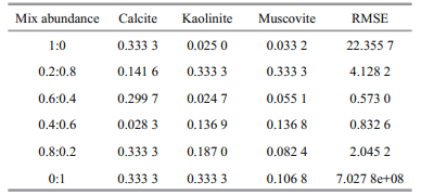
Spectra of three pure pixels correspond to minerals: calcite (red), kaolinite (green) and muscovite (blue) are in Fig. 2a. By the generation strategy of simulation hyperspectral image illustrated in Fig. 3, the original hyperspectral imagery cube was generated as shown in Fig. 4a, and the original abundance maps of the original spectra are illustrated in Fig. 5a-c. Respectively, Fig. 2b and Fig. 5d-f show the results of three extracted endmembers and three abundances in quantified maps of different ICs using the ICA algorithm. The change in order of the ICs can be observed. These need to be rearranged to determine which spectrum corresponds to each original mineral. By calculating the spectral angle shown in Table 1, we can find the correspondence between the original spectra and the extracted endmembers, and then adjust the ordering of the ICs. The resulting endmembers and abundances are illustrated in Fig. 2c and Fig. 5g-i. Figure 4d shows the position of ICs found by the ICA method. Using the abundance maps, we can reconstruct the hyperspectral image box, shown in Fig. 4b. To estimate the difference between the original image cube and the reconstructed image cube, the abundance error image was acquired as illustrated in Fig. 4c.


|
| Figure 5 Abundance maps |
The processing procedure example above illustrates how ICA works. To evaluate the performance of ICA, the total result of abundance estimation error (%) and root mean square error (RMSE) is tabulated in Table 2.
In this section, real hyperspectral image data were used for experiments. On 19 June, 2011, an actual marine oil spill occurred in the sea off Changdao, in Shandong Province, China. The North Sea aviation team of the State Oceanic Administration (People's Republic of China) collected hyperspectral data by helicopter, using a marine surveillance force and a push-broom hyperspectral imaging camera. The hyperspectral data are 256-band images with 400-1 100-nm spectral band ranges.
The helicopter flew at an altitude of 500 m and the image surficial spatial resolution was 2 m. Eight hyperspectral imagery scenes were collected. These are the original data for this experiment. At the same time, synchronous surficial hyperspectral data were also collected by ASD spectrometer. These spectra include sea water, oil spill and sun glint regions, as illustrated in Fig. 6b. The frequency range of the spectra is 400-1 100 nm, with 256 bands and the angle of view of the bare fiber is 25°. The results of one image are shown in Fig. 6a.

|
| Figure 6 Real hyperspectral imagery and original spectra of oil spill |
Figure 7a-c and Fig. 7d-f show the fractional abundances of sea water, oil spill and sun glint by NMF and ICA, respectively. The spatial location of the three pixels extracted in Fig. 6a by ICA is marked by a blue circle, and the corresponding three different endmembers are shown in Fig. 6b. To indicate the relationship of ICs and the original endmembers, a SAM was used for spectral identification. The synthetic data experiment showed that the SAM was the best spectral similarity measure for hyperspectral imagery. To adjust the orders of the ICs, SAM can measure the similarity of the endmembers extracted by ICA and the endmembers collected by ASD spectrometer. As a comparison, Fig. 7a-c shows the result obtained by the N-Finder and NMF. The oil spill endmember was can be observed as missing. Comparing the NMF result in Fig. 7a-c to the result produced in Fig. 7d-f by the ICA, the ICA performed better than the NMF. As illustrated in Fig. 7e, this atsea oil spill has obvious zonal distribution characteristics.

|
| Figure 7 Endmember abundance of one image |
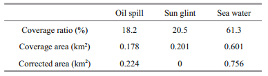
It should be noted that if we want to calculate the oil spill coverage area accurately, we need to know the oil spill abundance fraction for each pixel in the image. However, if we know the spatial resolution, we can estimate the approximate area covered by the oil. The abundance fraction is the proportion of coverage of the corresponding endmember. The results are tabulated in Table 3. The coverage ratio of this oil spill was 18.2%. The total area of the eight hyperspectral image scenes covered is 0.98 km2, which was calculated by multiplying the number of pixels by the spatial resolution. This simple method ignores one important issue: the sun glint area may conceal spilled oil. The proportion of oil in sun glint therefore needs to be calculated to correct the result. Because there are only water and oil on the sea surface, the percentage of oil area in sun glint can be calculated according to the probability of oil and water. As tabulated in Table 3, the corrected result is 0.224 km2. The corrected coverage ratio of oil spill is 22.89%, and there is a 2.11% deviation with the navigator's live estimate result, which is 25%.
Taking full account of the differences and similarity between spectra collected by ASD spectrometer and hyper-spectral data collected on aircraft, it conforms to spatial perceptive law in theory, and it can improve the efficiency of recognition given spectra of oil spill in technology. But in practice, it is difficult to estimate exact oil spill coverage rates, and information on this is lacking. It is therefore reasonable to use synthetic image-based computer simulations for performance analysis. Additionally, the existence of sun glint causes severe disruption for oil detection. It is therefore necessary to correct for sun glint before abundance detection. No standardized method is currently available for detecting oil in sun glint, so this paper makes a reasonable estimation of the oil spill by probability.
The effects of breaking waves on the sea surface, and the limitation of the ground resolution of airborne remote sensing, means that there is also no reliable method to estimate the exact abundance of oil spill in a single pixel of remote sensing imagery. This paper presents an abundance quantification method based on ICA for estimating the coverage rate of oil spills at sea. To calculate the area of oil spills covered accurately, we improved the ICA algorithm by adding constraint conditions. These are non-negativity and a constant sum. We followed this with priority weighting using higher-order statistics and the SAM method to overcome the order non-determinacy of ICs. Simulation and real data experiments were conducted using the algorithm above to estimate the coverage of a real oil spill and to validate our results. The method described in this paper can be used for the automatic monitoring of oil spills and accurate estimating of their area.
| Cococcioni M, Corucci L, Masini A, Nardelli F, 2012. SVME:an ensemble of support vector machines for detecting oil spills from full resolution MODIS images. Ocean Dynamics, 62(3): 449–467. Doi: 10.1007/s10236-011-0510-8 |
| Hyvärinen A, Karhunen J, Oja E, 2001. Independent Component Analysis. Wiley and Sons, New York476p. |
| Hyvärinen A, Oja E, 1997. A fast fixed-point algorithm for independent component analysis. Neural Computation, 9(7): 1483–1492. Doi: 10.1162/neco.1997.9.7.1483 |
| Jha M N, 2009. Development of Laser Fluorosensor Data Processing System and GIS Tools for Oil Spill Response. University of Calgary, Calgary, Alberta124p. |
| Keshava N, Mustard J F, 2002. Spectral unmixing. IEEE Signal Processing Magazine, 19(1): 44–57. Doi: 10.1109/79.974727 |
| Kessle J D, Valentine D L, Redmond M C, et al, 2011. A persistent oxygen anomaly reveals the fate of spilled methane in the deep Gulf of Mexico. Science, 331(6015): 312–315. Doi: 10.1126/science.1199697 |
| Lee D D, Seung H S, 1999. Learning the parts of objects by non-negative matrix factorization. Nature, 401(6755): 788–791. Doi: 10.1038/44565 |
| Leifer I, Lehr W J, Simecek-Beatty D, et al, 2012. State of the art satellite and airborne marine oil spill remote sensing:application to the BP Deepwater Horizon oil spill. Remote Sensing of Environment, 124: 185–209. Doi: 10.1016/j.rse.2012.03.024 |
| Lennon M, Babichenko S, Thomas N, et al, 2006. Detection and mapping of oil slicks in the sea by combined use of hyperspectral imagery and laser induced fluorescence. Earsel Eproceedings, 5(1): 120–128. |
| Lu Y C, Li X, Tian Q J, et al, 2013. Progress in marine oil spill optical remote sensing:detected targets, spectral response characteristics, and theories. Marine Geodesy, 36(3): 334–346. Doi: 10.1080/01490419.2013.793633 |
| Mirzal A, 2014. NMF versus ICA for blind source separation. Advances in Data Analysis and Classification: 1–24. Doi: 10.1007/s11634-014-0192-4 |
| Nascimento J M P, Dias J M B, 2005. Does independent component analysis play a role in unmixing hyperspectral data?. IEEE Transactions on Geoscience and Remote Sensing, 43(1): 175–187. Doi: 10.1109/TGRS.2004.839806 |
| Ramsey Ⅲ E, Rangoonwalaa A, Suzuoki Y, Jones C E, 2011. Oil detection in a coastal marsh with polarimetric synthetic aperture radar (SAR). Remote Sensing, 3(12): 2630–2662. Doi: 10.3390/rs3122630 |
| Srivastava H, Singh T P, 2010. Assessment and development of algorithms to detection of oil spills using MODIS data. Journal of the Indian Society of Remote Sensing, 38(1): 161–167. Doi: 10.1007/s12524-010-0007-9 |
| Wang J, Chang C I, 2006a. Applications of independent component analysis in endmember extraction and abundance quantification for hyperspectral imagery. IEEE Transactions on Geoscience and Remote Sensing, 44(9): 2601–2616. Doi: 10.1109/TGRS.2006.874135 |
| Wang J, Chang C I, 2006b. Independent component analysisbased dimensionality reduction with applications in hyperspectral image analysis. IEEE Transactions on Geoscience and Remote Sensing, 44(6): 1586–1600. Doi: 10.1109/TGRS.2005.863297 |
| Winter M E. 1999. N-FINDR: an algorithm for fast autonomous spectral end-member determination in hyperspectral data. In: SPIE's International Symposium on Optical Science, Engineering, and Instrumentation. International Society for Optics and Photonics. p. 266-275. |