 2017, Vol. 35
Institute of Oceanology, Chinese Academy of Sciences
Article Information
- LU Zaihua(卢再华), ZHANG Zhihong(张志宏), GU Jiannong(顾建农)
- Modeling of low-frequency seismic waves in a shallow sea using the staggered grid difference method
- Chinese Journal of Oceanology and Limnology, 35(5): 1010-1017
- http://dx.doi.org/10.1007/s00343-017-6026-4
Article History
- Received Feb. 1, 2016
- accepted in principle Apr. 5, 2016
- accepted for publication Jun. 28, 2016


When a ship or a submarine sails in a shallow sea, an elastic wave is usually generated on the seabed by the low-frequency noise of the ship. This type of elastic wave is commonly called 'ship seismic wave' and can be used to identify ships (Lu et al., 2004). Previous experimental studies investigated the transformation of underwater acoustic radiation into seismoacoustic waves (Averbakh et al., 2002; Dolgikh and Chupin, 2005). Theoretical modeling and analyses of seismic waves on the seafloor generated by lowfrequency sound waves were carried out using the normal mode model (Yan et al., 2006), fast field program (Lu et al., 2011) and parabolic equations (Zhang et al., 2010). These researchers focused on the propagating properties of seismic waves in the frequency domain by calculating transmission loss curves, frequency response curves, and so on. However, analysis in the frequency domain cannot distinguish accurately between the different components of the seismic waves. These components—P-waves, S-waves, normal modes, and interface waves—are important for our understanding of the propagating mechanism of ship seismic waves. A numerical simulation in the time domain of seismic waves generated by a low-frequency source is needed to analyze the wave components of ship seismic waves. The staggered-grid finite difference method was developed and is widely used to simulate seismic waves in the time domain (Zhang et al., 2008; Yang et al., 2012); however, little attention has been paid to seismic waves caused by low-frequency sound sources in shallow seas and in far-field cases. In this work, we first introduce an algorithm for simulating seismic waves at the seafloor in shallow water based on the staggered-grid finite difference method. Then we present numerical simulation of seismic waves caused by low-frequency sound waves from a point source in a typical shallow sea environment. The primary goal of this work is to establish a finitedifference scheme and demonstrate its effectiveness by analyzing the various types of ship seismic waves. The results of this work may serve as a guideline for other studies on similar wave phenomena.
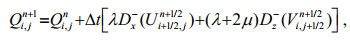
2 STAGGERED-GRID FINITE DIFFERENCE METHODTo model wave propagation in shallow water with a perfectly elastic, isotropic seabed, we follow the staggered-grid finite difference method proposed by Virieux (1986) and Graves (1996), which solves the following elastodynamic equations:
 (1)
(1) (2)
(2)where vi is the particle velocity component; τij is the stress tensor component; λ and μ are Lame's constants; ρ represents the medium density; and δij is the component of the Kronecker tensor; θ is the bulk strain.
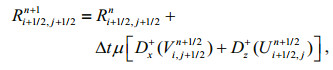
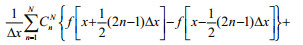
In this study, we only carried out a 2-dimensional (2D) analysis which is simpler than a 3-dimensional approach and can provide the primary propagation characteristic of seismic waves in a shallow sea generated by a low-frequency sound source. 2D analysis gives a qualitative representation of the wave processes only and does not evaluate the level of acoustic and bottom seismic waves quantitatively (especially in the case of a sloping bottom). The staggered grid defines some of the velocity and stress components shifted from the locations of other components by half a grid length in space as shown in Fig. 1. By using a second-order approximation for the time derivatives and tenth-order approximation for the spatial derivatives (Dong et al., 2000; Pei and Mu, 2003), the solutions of Eqs.1 and 2 can be expressed in discrete forms by:
 (3)
(3) (4)
(4) (5)
(5) (6)
(6) (7)
(7)

|
| Figure 1 Location of discretized variables and constants in the finite-difference cells |
where U and V are the discretized particle velocity variables vx and vz, and P, Q, and R are the discretized stress variables τxx, τzz, and τxz, respectively. In these equations, the superscripts refer to the time indices and the subscripts refer to the spatial indices, for example, 

In this article, the perfectly matched layer (PML) technology proposed by Collino and Sogka (2001) is applied to reduce the reflections from the artificial boundaries of the numerical model. The whole computational domain is divided into an interior region (white region) and PML regions (gray regions) as shown in Fig. 2.

|
| Figure 2 A shallow sea model for seismic waves generated by a point source The upper layer is sea water, 100 m deep and the bottom layer is seabed, 1 250 m in depth. |
For modeling a semi-infinite space, the free boundary condition is the stress-free condition at the free surface, requiring (τiz)z=0=0. We satisfy the free surface boundary condition by the zero-stress formulation of Graves (1996). If we assume symmetry for the stress components about z=0 and extend the grid several nodes above z=0, we can use the boundary condition to satisfy the free-surface condition. In Fig. 3, the zero-stress free-surface boundary is shown by the heavy solid line and coincides with the location of the normal stress nodes. Choosing the z axis as the vertical direction (positive downward) and setting the free surface at z=0, the following expression must be satisfied for the 2-D model:
 (8)
(8)

|
| Figure 3 Layout of the field variables for the zero-stress freesurface boundary |
Upon discretizing the model, certain values of the stress components need to be specified at and above the free-surface boundary to solve the interior system given by Eqs.3–7. Setting the free-surface boundary at iz=j (Fig. 3), the values of the stress field at and above the free surface are obtained using the antisymmetric property:
 (9)
(9) (10)
(10)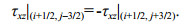 (11)
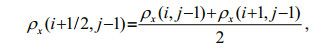
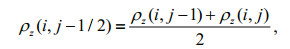
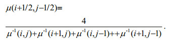
(11)At the seafloor interface, arithmetic averaging must be used for the density values, and harmonic averaging is required for the shear modulus (Graves, 1996). In Fig. 3, if we replace the zero-stress free surface with the seafloor interface, these averages can be represented by
 (12)
(12) (13)
(13) (14)
(14)The wave equation of the fluid layer can be derived from the elastodynamic equations (Eqs.1 and 2). We simply set ρ as the seawater density, μ=0, and substitute λ with the bulk modulus K=ρc2 of sea water (Shapiro et al., 2002).
For the numerical modeling, the time function of the source is given by,
 (15)
(15)where the variable f represents the vertical force or acoustic pressure in the following numerical examples; fc is the central frequency and tc describes the frequency bandwidth of the wavelet. A wavelet with fc=10 Hz and tc=0.2 s is shown in Fig. 4.

|
| Figure 4 Source wavelet with fc=10 Hz and tc=0.2 S |
To minimize the numerical dispersion and guarantee the accuracy of the staggered-grid finitedifference (FD) scheme, we selected a spatial discretization scheme that satisfies the following inequality (Pitarka, 1999),
 (16)
(16)where fmax is the maximum frequency of the propagating signal, vmin is the lowest velocity, and Δ is the grid spacing. A theoretical analysis of the stability condition of the proposed scheme is difficult to obtain; therefore, we adopted the stability condition of the staggered-grid scheme simplified for a constant grid spacing (Dong et al., 2000),
 (17)
(17) (18)
(18)where Δt is the time increment, and λ, μ are the Lame constants.
3 NUMERICAL EXAMPLESIn this study we performed two types of tests. Test 1 was designed to analyze the accuracy of the FD scheme with a vertical-force source in the seabed. In the second group of tests, sound sources located in the water were used to simulate the propagation of acoustic and seismic waves in a shallow sea.
3.1 Accuracy analysisTo assess the accuracy of the proposed staggeredgrid FD scheme, we modeled the wave propagation in a two-layered laterally homogeneous media (Fig. 2) (Test 1). The model is 1 250 m wide and 1 250 m deep. The spatial and temporal steps are Δx=Δz=5 m and Δt=1 ms. There are 10 cells of PML along the bottom and vertical sides of the computational domain. The source is a vertical force located at a depth of 575 m below the sea floor at the center of the model. The source function is a cosine envelope wavelet given by Eq.15 with a central frequency of 40 Hz and a bandwidth of 80 Hz. The upper layer is sea water with a depth of 100 m, vp=1 500 m/s, and ρ=1 000 kg/m3. The lower layer represents the seabed with vp=2 400 m/s, vs=1 600 m/s and ρ=1 800 kg/m3. The receiver is 300 m from the source in both the x and z directions. In this model the waveform at the receiver is equivalent to the waveform recorded in an infinite space before any reflected waves have reached the receiver. Thus, the analytic solutions in the time domain for a 2D unbound space with a vertical-force source given by Pilant (1979) can be used to test the accuracy of the FD scheme above.
 (19)
(19)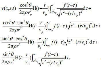 (20)
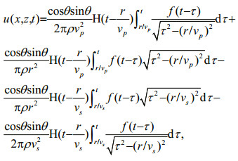
(20)where u(x, z, t) and v(x, z, t) are the horizontal and vertical displacements at location (x, z) and time t; vp and vs are the compressional and shear wave speeds; H represents the Heaviside function; f is the source wavelet function; r and θ are the distance and the azimuthal angle between the receiver and the source.
The numerical results based on the staggered-grid FD scheme agree well with the analytical solutions (Fig. 5), thus validating the staggered-grid FD method. The slight differences between the two solutions were caused by the numerical dispersion that occurred because the maximal frequency of the source was limited to 80 Hz. As most of the frequency of sound source in this study is very low and the wavelength is much wider than the grid size, the numerical dispersion in Test 1 will be relatively weak in other tests. Figure 6 shows a snapshot of the velocity component in the x-z plane at time 0.315 s. The source excites two direct waves that propagate through the seabed, a compressional wave P2 and a shear wave S2, where the subscript 2 indicates the sequence number of the layer in the half-space (1-water layer, 2-seabed layer). The horizontal velocities of the P-and S-waves in Fig. 6 are zero in the horizontal and vertical directions. This shape is coincident with Eq.19 where u(x, z, t) is antisymmetric about the horizontal and vertical directions. Similarly, the shape of the P-wave and the S-wave in Fig. 7 is symmetric about the horizontal and vertical directions according to the trigonometric functions in Eq.20.

|
| Figure 5 Waveforms at the receiver; staggered-grid FD scheme (grey line) and analytical solution (black line) a. horizontal velocity; b. vertical velocity. |

|
| Figure 6 Snapshot of horizontal velocity at t=0.315 s (fc=40 Hz) |

|
| Figure 7 Snapshot of vertical velocity at t=0.315 s (fc=40 Hz) |
The PML layers on the bottom and sides of the computational domain absorb the outgoing waves very well and spurious reflection is almost invisible. At t=0.315 s the upgoing direct wave P2 had interacted with the seafloor interface and produced a downgoing reflected compressional wave P2P2, a reflected shear wave P2S2 in the seabed, and an upgoing transmitted wave P2P1 in the sea water. The downgoing reflected wave P2P1P1 is produced from the transmitted wave P2P1 at the water surface. While both compressional and shear waves are generated in the sea bed layer, only compressional waves are generated in the water layer. The above propagation characteristics demonstrate that the numerical model presented here achieves good simulation of the artificial boundary, seafloor interface, and free surface.
3.2 Numerical simulation in the near-field caseBased on numerical Test 1, the forward numerical simulation of the seismic wave generated by a lowfrequency sound source in a shallow sea can be carried out if we replace the vertical force located in the seabed with a sound source located in the water and adjust the size of the computational domain accordingly (with the same grid size as in Test 1). The far-field case is defined as the situation where the source and the receiver or the interest area are separated by a distance that is more than ten times the depth of the water. In this case, most of the acoustic rays arriving at the receiver were reflected by the sea floor and sea surface many times, with the water layer acting as a waveguide. The near-field case occurs when the receiver or the interest area are separated from the source by a distance that is only a few times the depth of the water.
First, we calculated the seismic wave generated by a low-frequency sound source in a shallow sea for the near-field case (Test 2). Snapshots of the vertical component of the particle velocity at time 0.1 s and 0.125 s are shown in Figs. 8 and 9, respectively. The "+" symbol in Fig. 8 represents the sound source which is placed 20 m above the seafloor and has the same source function as in Test 1. Placing the source at a water depth of 80 m aims to simulate a submarine moving in shallow sea. At 0.1 s (Fig. 8), the source pulse labeled P1 has interacted with the seafloor and the sea surface. The upgoing reflected wave P1P1u and the downgoing reflected wave P1P1d were produced from the lower and upper boundaries of the water layer. In Fig. 8 we also observe two wavefronts in the seabed layer, namely, the transmitted compressional wave P1P2 and the transmitted shear wave P1S2 which are produced from the source pulse P1 when it hits the seafloor. At t=0.125 s (Fig. 9) the interface waves have propagated from the sea floor and their amplitudes decay rapidly away from the interface. The first seismic wave in the seabed is the low-amplitude compressional wave P1P2, followed by the transmitted shear wave P1S2 and the interface waves along the x direction. In the near-field case, the seismic waves in the seabed are composed mostly of the transmitted shear wave P1S2 and the interface waves.

|
| Figure 8 Snapshot of vertical velocity at t=0.1 s (fc=40 Hz) in the near field case (Test 2) |

|
| Figure 9 Snapshot of vertical velocity at t=0.125 s (fc=40 Hz) in the near field case (Test 2) |
In Test 3, we carried out forward numerical simulation of the seismic wave in the far-field case. The source pulse has a central frequency of 20 Hz and a bandwidth of 40 Hz. The computational domain is extended to 2 500 m in the horizontal direction. Figures 10 and 11 are snapshots of the horizontal and vertical velocity, respectively, in the x-z plane at 1.5 s. The source position in Test 3 is at x=0 m, z=80 m. We also added 30 cells on the left side of the sound source (to the left of x=0 m). This area is not included in the computational domain because it is used only to separate between the sound source and the left PML boundary. There are two distinct wave packets along the propagation direction in the snapshots. The wave packet at a range of about 1 800 m corresponds to the interface wave because its peak amplitude is highest along the seafloor with an exponentially decaying amplitude away from the guiding interface. The wave packet at the radial range of 2 000–2 300 m has a different pattern; the horizontal velocity reaches its maximum while the vertical velocity diminishes at the mid-depth of the water layer. Moreover, the horizontal velocity signal is in phase throughout the water column while the vertical velocity in the middle of the water column is in antiphase to the velocity in the lower and upper parts of the column. This corresponds exactly to the depth function of the first mode according to normal mode theory (Jensen et al., 1994; Li et al., 2000). Hence, the wave components of the seismic wave in the far-field case are mainly the normal mode and the interface wave caused by the waveguide effect of the sea water and the interface effect of the sea floor.

|
| Figure 10 Snapshot of horizontal velocity at t=1.5 s (fc=20 Hz) for the far-field case, Test 3 |

|
| Figure 11 Snapshot of vertical velocity at t=1.5 s (fc=20 Hz) for the far-field case, Test 3 |
To analyze the influence of the source frequency on the seismic wave in the far field, in Test 4 we reduced the central frequency of the source pulse to 10 Hz with a bandwidth of 20 Hz. Snapshots of the horizontal and vertical velocity are shown in Figs. 12 and 13, respectively. Compared with Figs. 10 and 11, the peak amplitude of the interface wave is higher while that of the normal mode is lower. This effect is also evident in the time series of the vertical velocity in Fig. 14 (fc=20 Hz) and Fig. 15 (fc=10 Hz). Thus, a lowfrequency source is favorable for generating interface waves in the far field. This propagation characteristic was analyzed by Lu et al. (2013) who derived the phase velocity dispersion curves for waves in a shallow sea. As shown in Fig. 16 (Lu et al., 2013), there are usually an interface wave and several normal modes displayed in the dispersion curves when the frequency range is below 100 Hz. Each normal mode has a well-defined low-frequency cutoff while the interface wave does not. Thus, the time series of the seismic wave is dominated by the interface wave when the source frequency is less than the minimal cut-off frequency of the normal modes ( < 20 Hz). Higher-order normal modes appear when the source frequency increases and gradually passes their cut-off frequencies (>20 Hz). The normal modes gradually become the dominant carriers of the source energy, and the interface wave weakens accordingly.

|
| Figure 12 Snapshot of horizontal velocity at t=1.5 s (fc=10 Hz) for low-frequency case, Test 4 |

|
| Figure 13 Snapshot of vertical velocity at t=1.5 s (fc=10 Hz) for low-frequency case, Test 4 |

|
| Figure 14 Time series of the vertical velocity at the seafloor r=1 400 m, fc=20 Hz. |

|
| Figure 15 Time series of the vertical velocity at the seafloor r=1 400 m, fc=10 Hz. |

|
| Figure 16 Phase velocity dispersion curves (Lu et al., 2013) |
To analyze the wave components and the propagation properties of ship seismic waves in a shallow sea, we developed an algorithm for simulating seismic waves at the seafloor based on the staggeredgrid finite difference method. Forward numerical simulations of seismic waves generated by a lowfrequency sound source in a shallow-water environment were carried out. Because the frequency of the sound-wave source in this work is very low and the bottom attenuation is relatively small compared with that of a high-frequency sound source, we ignored the dissipation losses in this simulation. Based on the results of the numerical simulations without bottom attenuation we can draw the following conclusions.
(1) The seismic waves in the near-field case are mostly composed of transmitted S-waves and interface waves while the transmitted P-waves are relatively weak near the seafloor.
(2) In the far-field case, the wave components of the seismic waves are mainly the normal modes and the interface waves.
(3) As the frequency of the source decreases, the peak amplitude of the interface wave increases while that of the normal mode decreases. Thus, a lowfrequency source is favorable for generating interface waves in the far field.
The wave components and the propagation properties of ship seismic waves in shallow water are discussed to some extent in this paper. The hydrogeology conditions in a shallow sea are complex; these include shallow water, negative sound-speed gradients, sloping sea bottom and poroelastic sediments. In this work we did not account for dissipation losses of the seismic wave propagation in the bottom medium. Wave absorption by propagation in the bottom medium is higher than in the water medium; this can affect the simulation results. Therefore, this effect should be incorporated in future studies on the propagation properties of ship seismic waves in a shallow sea.
| Averbakh V S, Bogolyubov B N, Dubovoi Y A, et al, 2002. Application of hydroacoustic radiators for the generation of seismic waves. Acoustical Physics, 48(2): 121–127. Doi: 10.1134/1.1460944 |
| Collino F, Sogka T, 2001. Application of the perfectly matched absorbing layer model to the linear elasto-dynamic problem in anisotropic hetero-geneous media. Geophysics, 66(1): 294–307. Doi: 10.1190/1.1444908 |
| Dolgikh G I, Chupin V A, 2005. Experimental estimate for the transformation of underwater acoustic radiation into a seismoacoustic wave. Acoustical Physics, 51(5): 538–542. Doi: 10.1134/1.2042572 |
| Dong L G, Ma Z T, Cao J Z, et al, 2000. A staggered-grid highorder difference method of one-order elastic wave equation. Chinese Journal of Geophysics, 43(3): 411–419. |
| Graves R W, 1996. Simulating seismic wave propagation in 3D elastic media using staggered-grid finite-differences. Bull. Seism. Soc. Am., 86(4): 1091–1106. |
| Jensen F B, Kuperman W, Porter M B, 1994. Computational Ocean Acoustics. AIP Press, New York. |
| Li Z L, Wang Y J, Ma L, et al, 2000. Effects of sediment parameters on the low frequency acoustic wave propagation in shallow water. Acta Acustica, 25(3): 242–247. |
| Lu Z H, Zhang Z H, Gu J N, 2004. The ship-induced seismic wave on the seafloor and it's application in water mine fuze. Mine Warfare and Ship Self-Defence(4): 25–28. |
| Lu Z H, Zhang Z H, Gu J N, 2011. An algorithm for seismic wave on seafloor caused by low frequency point sound source based on wave-number integration technique. Journal of Wuhan University of Technology(Transportation Science & Engineering), 35(1): 118–121. |
| Lu Z H, Zhang Z H, Gu J N, 2013. Numerical calculation of seafloor synthetic seismograms caused by low frequency point sound source. Defence Technology, 9(2): 98–104. Doi: 10.1016/j.dt.2012.12.001 |
| Pei Z L, Mu Y G, 2003. A staggered-grid high-order difference method for modeling seismic wave propagation in inhomogeneous media. Journal of the University of Petroleum, China, 27(6): 17–21. |
| Pilant W L. 1979. Elastic Waves in the Earth. Elsevier Press, Amsterdam. p. 59-63. |
| Pitarka A, 1999. 3D elastic finite-difference modeling of seismic motion using staggered grids with nonuniform spacing. Bull. Seism. Soc. Am., 89(1): 54–68. |
| Shapiro N M, Olsen K B, Sing S K, 2002. On the duration of seismic motion incident onto the Valley of Mexico for subduction zone earthquakes. Geophys. J. Int., 151(2): 501–510. Doi: 10.1046/j.1365-246X.2002.01789.x |
| Virieux J, 1986. P-SV wave propagation in heterogeneous media:velocity-stress finite-difference method. Geophysics, 51(4): 889–901. Doi: 10.1190/1.1442147 |
| Yan B, Zhou W, Gong S G, 2006. A normal mode model for ocean seismo-acoustics in shallow water. Journal of Wuhan University of Technology (Transportation Science & Engineering), 30(5): 804–806, 830. |
| Yang Z, Li R Y, Yue J G, et al, 2012. Seismic wave field numerical modeling with high-order finite-differential method. Journal of Beijing Jiaotong University, 36(5): 68–72, 83. |
| Zhang H G, Piao S C, Yang S E, 2010. Propagation of seismic waves caused by underwater infrasound. Journal of Harbin Engineering University, 31(7): 879–887. |
| Zhang H X, He B S, Zhang J, et al, 2008. Forward modeling of seismic wave fields in complex anisotropic media using finite difference method. Journal of China Coal Society, 33(11): 1257–1262. |