 2017, Vol. 35
Institute of Oceanology, Chinese Academy of Sciences
Article Information
- WEI Yuqiu(魏玉秋), LIU Haijiao(刘海娇), ZHANG Xiaodong(张晓东), XUE Bing(薛冰), MUNIR Sonia(MUNIRSonia), SUN Jun(孙军)
- Physicochemical conditions in affecting the distribution of spring phytoplankton community
- Chinese Journal of Oceanology and Limnology, 35(6): 1342-1361
- http://dx.doi.org/10.1007/s00343-017-6190-6
Article History
- Received Jul. 31, 2016
- accepted in principle Sep. 14, 2016
- accepted for publication Sep. 29, 2016


2 Tianjin Key Laboratory of Marine Resources and Chemistry, Tianjin University of Science and Technology, Tianjin 300457, China;
3 Institute of Marine Science and Technology, Shandong University, Jinan 250110, China
As primary producers in the marine ecosystem, phytoplankton play significant roles in food chains and global carbon cycle by photosynthesis providing energy for other organisms. Furthermore, phytoplankton cells are the main biological organism for seawater quality assessment attributing to their special responsive mechanism to surrounding environmental changes (Silva et al., 2005; Zhou et al., 2008). During the past several decades, most of the large estuaries and adjacent coastal oceans have been receiving numerous drainage waste products from riverine inputs. The phytoplankton in these environments are inevitably influenced by abundant loading nutrients (Dagg et al., 2004; Sun et al., 2010). Thus, phytoplankton cells concentrate and bloom frequently on continental shelves, where elevated amounts of nutrients are provided by anthropogenic input (Harrison et al., 2008; Guo et al., 2014). Overall, phytoplankton are generally spatially and temporally dynamic in community composition and distribution in such areas, where the strong interaction between rivers and oceans yields highly variable physical and chemical gradients (Zhu et al., 2009).
The Bohai Sea (BS) and Yellow Sea (YS) are significant semi-enclosed shelf seas of the northwest Pacific Ocean. Abundant discharges from the coastal currents carry a tremendous amount of eutrophic water with low temperature and salinity into the BS and YS, while the offshore oligotrophic water caused by the Kuroshio current is characterized by high temperature and salinity (Zhang et al., 2013). In spring, the BS and YS experience significant circulations and water masses, including the Bohai Sea Southern Coastal Water (BSSCW), Bohai Sea Mixed Water (BSMW), Yellow Sea Coastal Water (YSCW), Changjiang River Diluted Water (CRDW), Yellow Sea Cold Water Mass (YSCWM), Yellow Sea Warm Current (YSWC) and Kuroshio (Su and Weng, 1994; Jiang et al., 2015). Annually, owing to the large variation of both monsoons and circulations, water dynamics in the BS and YS vary greatly, which makes the hydrographic conditions in this area very complex (Zhao et al., 1994; Naimie et al., 2001). In the Bohai Sea, the phytoplankton community primarily concentrate near Huanghe (Yellow) River estuary, north of Bohai Bay and the Bohai strait. Annual variations of the phytoplankton distribution, however, have a close relationship with physical-chemical conditions in ambient waters (Sun et al., 2001). Wei et al. (2004) pointed out that the increased phytoplankton concentrations were observed in the Southern Bohai Sea in spring. In addition, the concentrations in coastal areas are higher than that in the Central Bohai Sea, which is strongly controlled by temperature, nutrient and especially by available light. In the Yellow Sea, nutrients come from the transportation of the Subei coastal water and the extension of the Changjiang (Yangtze) River diluted water. Under the influence of terrestrial runoff, high N/P ratios occur in the south and southwest of the Yellow Sea in spring. As a result, the primary production in a considerable portion of the Yellow Sea may be limited by phosphate rather than nitrogen (Wang et al., 2003). Moreover, Lin et al. (2005) displayed some other important responses of the Yellow Sea ecosystems to the changes in physical variables and chemical biogenic elements. These responses include decreasing phytoplankton abundance, succession of dominant species from diatoms to non-diatoms and changes in species diversity. Consequently, phytoplankton in the BS and YS exhibit complex spatio-temporal heterogeneity, which varies with the highly variable environmental conditions (Margalef, 1978; Hall et al., 2015).
Previous investigations of the environmental factors regulating phytoplankton community have been carried out for several decades. However, the physicochemical conditions in affecting regional distribution of phytoplankton community are still not fully understood. In this study, the phytoplankton in the BS and YS exhibited complicated regional distribution during spring. To understand more clearly the effects of physicochemical conditions on the regional distribution of phytoplankton community, we investigated the spatial distribution and biodiversity of phytoplankton and classified the phytoplankton community into 6 ecological provinces according to Multidimensional scaling (MDS) and cluster analysis. Furthermore, combined with our data of water temperature and salinity in the YS and BS, the various water masses and circulations were determined by T-S (temperature and salinity) scatter diagram. We examined how highly variable circulations and water masses (particularly the BSSCW, YSCW, CRDW, YSCWM and YSWC) control the spring phytoplankton community (abundance, dominant species and composition).
2 MATERIAL AND METHOD 2.1 Sampling and analysis methodsA comprehensive investigation was carried out in the BS and YS (31.3°–39.5°N, 118.9°–125.3°E). A total of 353 water samples from 110 stations were investigated as shown in Fig. 1.

|
| Figure 1 Location of sampling stations |
Water samples at different depths (surface [2 m], 5, 15, 25, 35, 45, 55, 65 m and bottom) from each station were collected by a Rosette sample system equipped with a CTD (SBE 917 Plus, Seabird Co.); temperature, salinity, depth and pressure were recorded at the same time. Water samples for phytoplankton analysis were fixed with 2% buffered formalin and stored in darkness. After returning to the laboratory, preserved samples were concentrated with 100 mL settlement columns for 24 to 48 h. And then, the phytoplankton taxa (cell size > 5 μm) were identified and counted under an inverted microscope (Motic BA300) at 400× (or 200×) magnification according to the methodology described by Utermöhl (1931).
Water samples for nutrient analysis were filtered through 0.45 μm cellulose acetate membrane filters and then refrigerated at 4℃ for further analysis. Nutrient concentrations including ammonium, phosphate, nitrate and silicate were determined by performing a Technicon AA3 Auto-Analyzer (Bran+Luebbe) according to classical colorimetric methods. The nitrate and ammonia concentrations were analyzed using the copper-cadmium column reduction method and the indophenol blue spectrophotometric method, respectively. Dissolved inorganic phosphorus (DIP) and silica (DSi) were measured using typical spectrophotometric methods (Pai et al., 2001; Dai et al., 2008; Guo et al., 2014).
2.2 Data analysis and statistical methodsDominance index (Y) was calculated to describe the species dominance in the phytoplankton community. The calculation equation was shown as follows:

N is the total number of individuals in the collected samples; ni is the cell number of species i; fi is the frequency of occurrence of species i in each sample (Sun and Liu, 2003). However, only the species that ranked in the top twenty dominances were considered the dominant species in the BS and YS. Multidimensional scaling (MDS) and cluster analysis were performed using PRIMER 6.0 to reveal spatial patterns in the community structure (Clarke and Gorley, 2001). Species abundance were transformed by Square roo t and standardized estimating Bra-Curtis similarities between sample pairs. To prevent the effects of rare species on the community, species having a dominance index (Y) < 0.09% were arbitrarily excluded in MDS and cluster analysis. Canonical Correspondence Analysis (CCA) was performed using MVSP software (v 3.1.3), and was applied on log(x+1)-transformed phytoplankton abundance and environmental data to determine the effects of environmental parameters on the community structure (Sun et al., 2014). Figures depicting horizontal and vertical distributions of phytoplankton abundance were constructed using Ocean Data View (4.6.7) and Grapher 10, respectively.
3 RESULT 3.1 Environmental parametersThe measured temperature and salinity in surface water were illustrated in Fig. 2. Water temperature ranged from 2.35℃ to 16.66℃ (mean=(9.87±3.00)℃). Low temperature was observed along the coasts of the BS and Northern Yellow Sea (NYS), indicating the waters there were affected by coastal currents. No significant difference in temperature was observed throughout the Southern Yellow Sea (SYS). However, small-scale temperature differences were found in the BS and NYS, which were mainly driven by the decrease in solar irradiation with latitude, coastal runoffs and the YSCWM. Sea surface salinity values (mean=31.68±1.14) varied between 26.89 and 33.89. No obvious difference in salinity was found in the open YS. In contrast, the cold water with low salinity were observed along the large estuaries and adjacent coastal oceans. For example, the Southern of Liaodong Peninsula and Changjiang River estuary were influenced by their diluted waters with low salinity and temperature.

|
| Figure 2 Horizontal distribution of (a) temperature (℃) and (b) salinity in the surface layers |
In the surface layers, high concentrations of ammonium, phosphate, nitrate and silicate occurred frequently along the offshore waters. Furthermore, the silicate concentration exhibited another relatively high level in oligotrophic open sea of SYS, and high phosphate level was also seen around the region of Northern Korea Bay (Fig. 3).

|
| Figure 3 Horizontal distribution of (a) ammonium, (b) phosphate, (c) nitrate and (d) silicate (μmol/L) in the surface layers |
The range and mean values of nutrient concentrations were shown in Table 1. Total ammonium value ranged from 0.01 to 3.59 μmol/L. The average values of ammonium concentration of three seas (BS, NYS and SYS) were (1.21±0.87) μmol/L, (0.95±0.78) μmol/L and (0.49±0.41) μmol/L, respectively, indicating the ammonium concentration in the BS was slightly higher than those in the NYS and SYS. Phosphate concentration remained consistently low throughout the studied area ( < 0.66 μmol/L). The relatively high concentration of phosphate mainly occurred in the central of the BS, Korean Peninsula coastal sea and Changjiang River estuary. However, the phosphate concentration was lower in the BS ( < 0.49 μmol/L) than in the NYS and SYS. Nitrate concentration ranged from 0.10 to 39.00 μmol/L. The nitrate concentration in the BS ((11.49±11.48) μmol/L) was predictably higher than in the NYS and SYS ((2.50±2.31) and (6.30±6.52) μmol/L, respectively). Inversely, the maximum average value of silicate concentration was (6.85±4.53) μmol/L occurring in the SYS.

A total of 162 phytoplankton taxa were identified during this survey. Bacillariophyta represented the most diverse group, and 105 diatom species were identified, representing 64.81% of the total taxa. Pyrrophyta was the second most diverse group (54 species), representing 33.33% of the total taxa. Species in other groups were recorded more sporadically, including 1 taxon in 1 genus of Chrysophyta (Dictyocha fibula) and 2 taxa in 2 genera of Chlorophyta (Scenedesmus quadricauda and Pediastrum duplex, respectively).
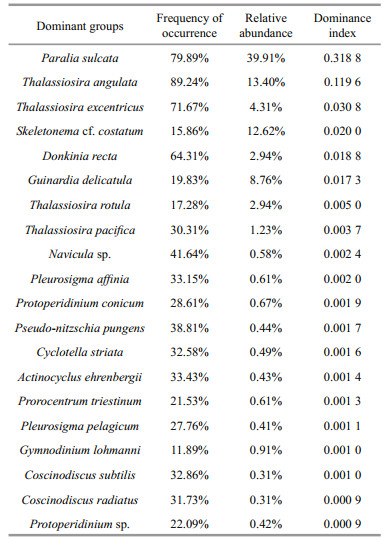
Phytoplankton abundance in the BS and YS ranged from 10 to (4.62×10⁴) cells/L, with an average value of (3.84×10³) cells/L. Diatoms were the most abundant group, accounting for 93.99% of the total phytoplankton abundance. Dinoflagellates generally occurred in low numbers, representing 5.74% of the total cell abundance. Another two groups similarly occurred at low abundance, representing only 0.27% of the total cell abundance. Overall, the phytoplankton assemblages were characterized by a great abundance of diatoms. The dominant groups of phytoplankton were obtained by calculating the index of dominance (Table 2).
The horizontal distribution of phytoplankton, diatoms and dinoflagellates were showed in Fig. 4. The surface abundance of phytoplankton ranged from 10 to (1.88×10⁴) cells/L, with an average value of (2.15×10³) cells/L. High abundance zones of phytoplankton were found in the central part of the BS, Korean Peninsula coastal sea, Lubei coastal area and Changjiang River estuary. The subsurface abundance ranged from 20 to (4.67×10⁴) cells/L, with an average value of (4.21×10³) cells/L. The bottom abundance varied between 10 and (4.64×10⁴) cells/L, with average value at (5.26×10³) cells/L. The abundance distribution patterns in the subsurface layers were similar to those in the bottom layers, Furthermore, phytoplankton abundance in the subsurface and bottom layers were obviously higher than that observed in the surface layers.

|
| Figure 4 Horizontal distribution of different phytoplankton taxonomic abundance (cells/L) in the surface, subsurface and bottom layers a, d, g. phytoplankton; b, e, h. diatoms; c, f, i. dinoflagellates. |
The concentrated zones of phytoplankton abundance were depicted by diatoms. The average abundances of diatoms in the surface, subsurface and bottom layers were (1.75×10³) cells/L, (4.07×10³) cells/L and (5.14×10³) cells/L, respectively. These abundance values had a trend of increase from surface layers to bottom layers. The average abundances of dinoflagellates in the surface, subsurface and bottom layers were (3.85×10²) cells/L, (1.29×10²) cells/L and (1.07×10²) cells/L, respectively. Conversely, dinoflagellates in low abundance was observed in the subsurface and bottom layers. High abundance zones of dinoflagellates only appeared in the surface layers of Shandong Peninsula, Southern of Liaodong Peninsula and Changjiang River estuary.
Figure 5 showed the horizontal distribution of dominant groups in the surface layers. The dominant groups were mainly comprised of diatoms. Paralia sulcata and Thalassiosira angulata were the most dominant species, with the dominances of above 31% and 11%, respectively (Table 2). P. sulcata primarily distributed around the Shandong Peninsula. The abundance of P. Sulcata ranged from 20 to (2.57×10⁴) cells/L, with an average value of (2.03×10³) cells/L. The abundance of T. angulata varied between 10 and (2.19×10⁴) cells/L, with an average value of (6.15×10²) cells/L. Meanwhile, the high abundance zones of T. angulata were mainly observed in north point of the survey area. The maximum abundance of Thalassiosira excentricus ((4.06×10³) cells/L) was found at Station B44. Skeletonema cf. costatum presented obviously ribbon distribution and dominated in the near-shore waters. The maximum abundance of S. costatum ((4.67×10⁴) cells/L) was observed at Station H37 nearby the Changjiang River estuary. The abundance of Donkinia recta varied from 10 to (1.52×10⁴) cells/L, and was mainly found in the coastal zones. Eventually, Guinardia delicatula was abundant at the stations of the BS and Lubei coastal areas.

|
| Figure 5 Horizontal distribution of dominant species in the surface layers (cells/L) a. Paralia sulcata; b. Thalassiosira angulata; c. Thalassiosira excentricus; d. Skeletonema cf. costatum; e. Donkinia recta; f. Guinardia delicatula. |
The vertical distribution of total phytoplankton abundance presented an apparent layering phenomenon. The total phytoplankton abundance increased gradually from 5 to 25 m depth and reached the maximum at depths of 25 m. Thereafter, it showed a relatively low abundance at 35 m depth, and then slightly increased from 35 to 55 m depth. Finally, the abundance dropped to minimum in the bottom layer. The vertical distribution of diatoms abundance showed a similar trend with the total phytoplankton, both reaching the maximum at depths of 25 and 55 m. Nevertheless, the high value of dinoflagellates abundance mainly distributed in the upper layer and reduced from 5 to 55 m depth obviously. The vertical distributions of dominant species, including P. sulcata, T. angulata, T. excentricus and D. recta, also showed the maximum abundance in the subsurface, as well as the depth of 45–55 m. However, the vertical distribution of S. costatum and G. delicatula scattered irregularly and unevenly throughout the whole water columns (Fig. 6).

|
| Figure 6 Vertical distribution of different phytoplankton taxonomic abundance (cells/L) a. phytoplankton; b. diatoms; c. dinoflagellates; d. Paralia sulcata; e. Thalassiosira angulata; f. Thalassiosira excentricus; g. Skeletonema cf. costatum; h. Donkinia recta; i. Guinardia delicatula. |
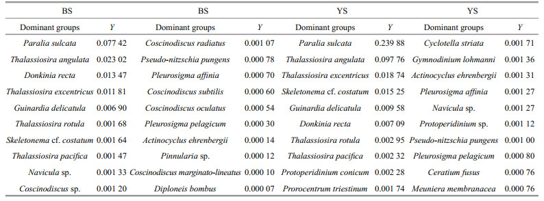
The dominants of phytoplankton in the BS and YS were showed respectively in Table 3. According to the top twenty dominants with stations as biological factors, the phytoplankton community could be classified into 6 ecological provinces based on MDS and cluster analysis. Phytoplankton community in the BS and YS were classified into 2 and 4 ecological provinces, respectively (Figs. 7, 8). A few specific stations distributed in overlapping groups or formed a unit by themselves. Anyway, combined with the various water masses and circulations, these specific stations were artificially divided into different ecological provinces (Fig. 9). In addition, Stations H45, H47, H08, H09 and H19 could not be classified into six provinces owing to the composition of the first twenty dominants in these stations showed a significant difference.

|
| Figure 7 MDS (left) and cluster analysis (right) of the top twenty dominants with stations in the BS Transform: square root; resemblance: S17 Bray Curtis similarity; 2D stress: 0.17. |

|
| Figure 8 MDS (a) and cluster analysis (b) of the top twenty dominants with stations in the YS Transform: square root; resemblance: S17 Bray Curtis similarity; 2D stress: 0.13. |

|
| Figure 9 Ecological provinces of phytoplankton community in the studied area |
The characteristics of six ecological provinces were showed in Table 4. Province Ⅰ (P-Ⅰ) consisted of 10 stations and located in the central part of the BS. The average values of temperature and salinity were 9.4℃ and 31.1, respectively. About 45 taxa of 4 phyla, including 36 taxa of Bacillariophyta, 6 taxa of Pyrrhophyta, 1 taxon of Chrysophyta and 2 taxa of Chlorophyta were found in P-Ⅰ. The total phytoplankton abundance ranged from 10 to (2.04× 10⁴) cells/L, and averaged at (6.43×10³) cells/L. Diatoms were the most abundant group, accounting for 99.80% of the total phytoplankton abundance. The dominant species in P-Ⅰ were mainly composed of P. sulcata, G. delicatula, D. recta, T. angulata, T. excentricus and S. costatum etc.
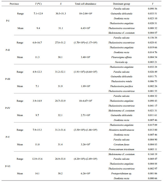
Province Ⅱ (P-Ⅱ) consisted of 14 stations and occurred around the BS. The mean values of temperature and salinity were 11.3℃ and 30.1, respectively. Thus, this ecological province belonged to a temperate semi-enclosed coastal sea. More than 58 taxa were identified from Bacillariophyta (50 taxa), Pyrrhophyta (7 taxa) and Chrysophyta (1 taxon). The total phytoplankton abundance varied between (1.70×10²) to (1.17×10⁴) cells/L, with an average value of (3.40×10³) cells/L. Diatoms accounted for 99.40% of the total phytoplankton abundance and were dominated by P. sulcata, T. excentricus, T. angulata, D. recta, P. affinia and Navicula sp. etc.
Province Ⅲ (P-Ⅲ) situated near the Northern Korea Bay. Temperature and salinity were recorded with the average values of 7.1℃ and 31.9, respectively. The temperature and salinity in P-Ⅲ were affected by the runoffs of the Northern Korea. Furthermore, the waters in P-Ⅲ were concurrently influenced by the YSCWM. Total 63 taxa were observed from Bacillariophyta (39 taxa), Pyrrhophyta (22 taxa), Chrysophyta (1 taxon) and Chlorophyta (1 taxon). The total phytoplankton abundance ranged from (1.91×10³) to (4.64×10⁴) cells/L, and the average value was (1.89×10⁴) cells/L. Diatoms represented about 97.76% of the total phytoplankton abundance and were dominated by T. angulata, P. sulcata, G. delicatula, T. rotula, T. pacifica and T. excentricus etc.
Province Ⅳ (P-Ⅳ) mainly located in the YS basin. The temperature varied from 3.9 to 14.9℃, presenting a significant difference. The temperature increased from north to south due to the increase in solar irradiation and warm-water intrusion. The mean value of salinity (32.1) exhibited a relatively high level, indicating the water in P-Ⅳ was drastically influenced by the YSCWM and an intrusion of the YSWC. Total of 127 taxa were identified from Bacillariophyta (83 taxa), Pyrrhophyta (42 taxa), Chrysophyta (1 taxon) and Chlorophyta (1 taxon). The total phytoplankton abundance ranged between 10 and (4.67×10⁴) cells/L, with an average value of (2.71×10³) cells/L. Diatoms accounted for 93.92% of the total phytoplankton abundance and were dominated by P. sulcata, T. angulata, T. excentricus, S. costatum, G. delicatula and D. recta etc.
Province Ⅴ (P-Ⅴ) consisted of 7 stations and located at coastal sites of the Western Yellow Sea. The average value of temperature was 11.0℃. Thus, this ecological province belonged to temperate coastal sea. The salinity was low and primarily caused by the YS coastal currents. The temperature decreased from coast to offshore gradually along the latitude because of the YSCWM. Total of 75 taxa were identified from Bacillariophyta (43 taxa), Pyrrhophyta (29 taxa), Chrysophyta (1 taxon) and Chlorophyta (2 taxa). The total phytoplankton abundance varied from (3.50×10²) to (1.46×10⁴) cells/L, with an average value of (3.26×10³) cells/L. This area was dominated by diatom species e.g., T. angulata, M. membranacea, D. recta, P. sulcata and dinoflagellate species e.g., C. fusus, P. triestinum etc.
Province Ⅵ (P-Ⅵ) situated at the southwest coastal area. Low salinity (30.2) was observed near the Changjiang River estuary, apparently indicating P-Ⅵ was affected by the Changjiang River. Additionally, strange solar irradiance in low latitudes promoted the light penetration, thereby the average temperature (14.1℃) was high. About 53 taxa were identified from Bacillariophyta (34 taxa), Pyrrhophyta (18 taxa) and Chrysophyta (1 taxon). Total phytoplankton abundance ranged from (4.20×10²) to (2.49×10⁴) cells/L, with an average value of (6.26×10³) cells/L. This province was dominated by diatom species e.g., S. costatum, P. sulcata, T. angulata, T. excentricus, D. recta and dinoflagellate species e.g., Protoperidinium sp. etc.
3.6 Phytoplankton abundance in relation to environmentCanonical correspondence analysis (CCA) was applied on 255 cases of the first twenty dominants and 7 environmental variables to determine the effects of environmental parameters on the phytoplankton community. Eigenvalues of CCA axis 1 and axis 2 were 0.094 and 0.049 separately, and the spec.-env. correlation coefficient were 0.663 and 0.668. The correlation coefficient of environmental axis 1 and axis 2 was 0, indicating that the degree of linear combination of CCA axis and environmental factors could properly reflect the relationship between dominants and environmental factors. Thus, the ordination results were reliable. Figure 10 showed CCA ordination of phytoplankton community with environmental variables in the BS and YS. The nutrients, light (pressure), temperature and salinity were the main variables affecting the phytoplankton community distribution. To clearly describe the relationship between the phytoplankton community and environmental factors, the phytoplankton community can be classified into several groups according to CCA.

|
| Figure 10 CCA ordination of phytoplankton community with environmental variables in the BS and YS PS: Paralia sulcata; TA: Thalassiosira angulata; TE: Thalassiosira excentricus; SC: Skeletonema cf. costatum; DR: Donkinia recta; GD: Guinardia delicatula; TR: Thalassiosira rotula; TP: Thalassiosira pacifica; NA: Navicula sp.; PA: Pleurosigma affinia; PC: Protoperidinium conicum; NP: Pseudonitzschia pungens; CS: Cyclotella striata; AE: Actinocyclus ehrenbergii; PT: Prorocentrum triestinum; PP: Pleurosigma pelagicum; GL: Gymnodinium lohmanni; CS: Coscinodiscus subtilis; CR: Coscinodiscus radiatus; PR: Protoperidinium sp. |
Group Ⅰ: phytoplankton in this group generally dominated in the open ocean, where the water was influenced by the YSWC. The temperature and salinity were high, while the nutrients concentration was low. These phytoplanktonic growth were favored by the increased temperature and salinity; Group Ⅱ: phytoplankton around the center of bi-plots mostly preferred high temperature, salinity and silicate; Group Ⅲ: phytoplankton preferred high salinity, relatively low levels of nutrients and temperature in shallow waters; Group Ⅳ: these phytoplankton mostly profited from coastal currents in condition with high nutrients, low temperature and salinity; Group Ⅴ: the primary environmental factor affecting the distribution of phytoplankton was nitrate, and the correlation was positive. It fitted to the condition of P-Ⅵ, which was influenced by Changjiang River with relatively low temperature and salinity.
4 DISCUSSION 4.1 Controlling factors of spring phytoplankton communityPhytoplankton community was mainly contributed by diatoms and dinoflagellates, and diatoms dominated throughout the BS and YS (Table 2). However, dinoflagellates showed higher frequency in the YS (Table 3). Nutrients availability was essential for phytoplanktonic growth and distribution (Fig. 10), which agreed with the previous nutrient analysis (Struyf et al., 2009). Numerous studies have demonstrated that structural and functional changes of the ecosystem in the BS and YS, such as changes in community composition and species abundance, were primarily caused by the increase of pollution and eutrophication (Lin et al., 2005; Gao et al., 2014). There was approximately one billion tons of sewage discharging from surrounding cities into the BS every year (Duan et al., 2010). Accordingly, the BS had one of the most eutrophic environments in China. The average nitrate and ammonium concentrations (11.49 and 1.21 μmol/L, respectively) in the BS were obviously higher than in the YS (table 1). Our CCA analysis revealed that diatoms correlated positively with the nitrate and ammonium (Fig. 10), indicating that high nitrate and ammonium favored the growth of diatoms. Concurrently, with yearly increases of nutrients and pollution, the annual bloom of diatoms occurred frequently in spring. Therefore, diatoms have a survival advantage over dinoflagellates in eutrophic waters. Research data have revealed that the phytoplanktonic growth was strongly dependent on the stabilization of water column (Margalef, 1978). The maximum averaged wave height was more than 1.05 m in the BS, and the wave directions varied significantly during spring (Lv et al., 2014). In particular, the wave turbulence has been reported to damage dinoflagellate cellular integrity and metabolism (Smayda, 1980). However, diatoms could thrive in strong turbulence due to the protection from their silicified cell walls (Hamm et al., 2003). In contrast, dinoflagellates were more susceptible to wave turbulence (Thomas and Gibson, 1990). Thus, the wave turbulence might be another limiting factor for the growth of dinoflagellates in the BS.
Previous studies revealed that the composition of phytoplankton community was closely related to the variable circulations and water masses (Liu et al., 2004). Yang et al. (2011) declared that the Kuroshio branches were significant drivers of the biogeochemical cycles in the East and South China Seas. Therefore, the YS in spring was mainly controlled by the YSWC, CRDW, YSCWM and Coastal runoffs (Jiang et al., 2015). The dominant dinoflagellates, e.g., Protoperidinium conicum, Prorocentrum triestinum, Protoperidinium sp. and Gymnodinium lohmanni preferred high temperature and salinity and relatively low levels of nutrients (Fig. 10). The resistance to starvation affected Protoperidinium's energy allocation and facilitated the dominance of Protoperidinium species in low nutrient levels (Menden-Deuer et al., 2005). Different water masses and circulations in the YS and BS were determined by the salinity and temperature properties (Su and Yuan, 2005). Combined with the water masses and various circulations, our data of water temperature and salinity of the YS and BS were analyzed to draw T-S (Temperature and Salinity) scatter diagram as shown in Fig. 11. The T-S diagram analysis suggested that the relatively high temperature and salinity appeared in the YSWC. Furthermore, Chen (2009) proposed that the YSWC originated from the Kuroshio and Taiwan Warm Current with poor nutrients concentration. By contrast, these observations led us to speculate that the dinoflagellates with high frequency in the YS might be transported from the YSWC.

|
| Figure 11 Temperature-Salinity (water masses) scatter diagram in the BS and YS a. BS; b. YS. BSSCW: Bohai Sea Southern Coastal Water; BSMW: Bohai Sea Mixed Water; CRDW: Changjiang River Diluted Water; YSCW: Yellow Sea Coastal Water; YSCWM: Yellow Sea Cold Water Mass; YSWC: Yellow Sea Warm Current. |
Some research showed the distribution and abundance of phytoplankton were controlled by the combined effects of several environmental parameters, generally including wave turbulence, nutrients, temperature, salinity and light availability (Chen et al., 2003; Luan et al., 2006). According to our CCA analysis, the abundance of dominant diatoms, belonging to Group Ⅳ and Group Ⅴ, correlated positively with nutrient concentrations, while negatively with temperature and salinity. This indicated that low nutrient level was a significant limiting factor for the growth of diatoms (Fig. 10). Furthermore, Fig. 11 showed the BSSCW, CRDW and YSCW had a significant function in controlling hydrological properties in seacoast, where the waters were characterized by low levels of temperature and salinity. Therefore, High abundance zones of diatoms in estuaries and coasts were affected by the runoffs. Since the 1980s, N :P ratio in marginal sea showed a trend of rising and Si:P ratio almost fell to the ecological threshold according to the Redfield ratio of 16:1 (N:P) (Lin et al., 2005). Richardson (1997) pointed out that when P was deficient and N was sufficient, the dominants of phytoplankton community would change from diatoms to dinoflagellates. Studies of Lake Michigan indicated that the addition of an external nutrient supply, high in N and P but low in Si, resulted in increased primary productivity (Schelske and Stoermer, 1971). From these points of view, we concluded that the phosphate concentration was the key limiting factor for diatoms growth. The phosphate concentration less than 0.2 μmol/L was very low, and near the ecological threshold essential for diatoms growth (Zou et al., 1983; Yu et al., 2000). Similarly, the phosphate concentration was deficient in the BS, NYS and SYS, with the average values of 0.12 μmol/L, 0.18 μmol/L, 0.20 μmol/L, respectively (Table 1). Consequently, phosphate tended to be the control factor for the horizontal distribution of diatoms abundance in spring.
P. sulcata and T. excentricus, belonging to Group Ⅳ, showed a positive correlation with nutrient levels and light availability (Fig. 10). P. sulcata was a brackish to marine diatom and commonly observed in the benthos of coastal waters (Zong, 1997; McQuoid and Hobson, 1998). Water columns vertical mixing had more upwelling of nutrient-rich to the surface, which subsequently resulted in high abundance of P. sulcata (McQuoid and Nordberg, 2003). Hence, P. sulcata was a frequently dominant species in spring, with the dominance of 0.077 42 and 0.239 88 in the BS and YS, respectively (Table 3). However, its abundance distribution in horizontal direction was controlled by phosphate concentration. An obvious correlation was observed between T. excentricus and light availability (Fig. 10). Jenkin (1937) pointed out T. excentricus, with its well-marked inhibition at illumination intensities, was only abundant in winter or early spring. In fact, in early spring or winter, the average amount of diurnal light reaching the surface waters was about one-ninth of that in a summer day, therefore, there would be no inhibition in growth of T. excentricus (Lebour et al., 1930). Moreover, there was less limitation for T. excentricus growth because of the sufficient nutrient materials in early spring. Thus, T. excentricus was another dominants in spring. T. angulata and G. delicatula belonging to Group Ⅱ showed positive corrections with temperature (Fig. 10), indicating they were suitable for growth in warm waters. T. angulata and G. delicatula would be abundant in low-latitude open seas, where stronger solar irradiance promoted the light penetration and provided a relatively warm seawater. Actually, Group Ⅱ around the center of bi-plots were mostly composed of eurythermal and euryhaline species, which were more tolerant to environmental stress according to CCA analysis. Consequently, high concentrated zones of T. angulata and G. delicatula were possibly distributed in northern coasts. Many occurrence of spring blooms were contributed by T. angulata and G. delicatula, including the coastal zones of Loch Creran (Harris et al., 1995), Northfrisian Wadden Sea (Tillmann et al., 1999) and Southern Bay of Biscay (Varela et al., 2006). S. costatum and D. recta belonging to Group Ⅴ were closely associated with nitrate, while negative correlation with temperature and salinity (Fig. 10). S. costatum, a well-known red tide species, was characterized by small size, high growth rate and nutrient uptake. Consequently, it had the advantages for growth in the nutrient replenishment (Tilman et al., 1981). The widespread occurrence of D. recta along the coasts was primary ascribed to the difference in vegetative structure and chloroplast division (Cox, 1981). In conclusion, S. costatum and D. recta had advantages in coastal waters due to their own strategies on nutrient utilization, vegetative and reproductive structure.
The vertical distribution of phytoplankton showed that the maximum abundance generally occurred in the subsurface (Fig. 6). However, the nutrients and light penetration were the key limiting factors for phytoplankton growth (Fig. 10). Smetacek (1985) proposed that phytoplankton often gathered in high light intensity and nutrient-rich water layers. Additionally, according to Klausmeier and Litchman (2001), light was supplied from surface and nutrients were often supplied from bottom, which were often the dilemma of living of phytoplankton. Consequently, phytoplankton concentrated in the subsurface because the light intensity was the optimal condition for phytoplankton growth. Moreover, zooplanktons mainly thrived in the depth less than 20 m water columns, which was another regulatory factor for phytoplankton distribution (Liu et al., 2015). Interestingly, another peak value occurred in the depth of 45–55 m. Although the light limitation suppressed the phytoplankton growth in deeper water column, nutrient levels supplying from bottom were relatively high and promoted the phytoplankton growth.
4.3 Relationship between ecological provinces and environmental conditionsPhytoplankton community in the BS and YS had complex composition and distribution, including freshwater, brackish, oceanic, benthic species, as well as eurythermal and euryhaline species. Water temperature and salinity were classified into six subregions according to the spatial variability in hydrological conditions namely, the BSSCW and BSMW in the BS, and the CRDW, YSWC, YSCW and YSCWM in the YS (Fig. 12). The pattern of hydrological partition was generally similar to the biological provinces. Consequently, we indicated that the different species composition and distribution were mainly influenced by various water masses and circulations. However, the analysis of ecological provinces could more accurately reflect the physicochemical conditions in affecting regional distribution of phytoplankton community.

|
| Figure 12 Different partitions of phytoplankton and hydrological conditions Red line represented phytoplanktonic partition and black line represented hydrological partition. BSSCW: Bohai Sea Southern Coastal Water; BSMW: Bohai Sea Mixed Water; CRDW: Changjiang River Diluted Water; YSCW: Yellow Sea Coastal Water; YSCWM: Yellow Sea Cold Water Mass; YSWC: Yellow Sea Warm Current. |
The community composition of the first six dominants in P-Ⅰ was similar to that in P-Ⅱ. However, the average abundance of phytoplankton in P-Ⅰ ((6.43×10³) cells/L) was nearly twice as large as in P-Ⅱ ((3.40×10³) cells/L) (Table 4). P-Ⅰ and P-Ⅱ could validly represent most parts of the BS. P-Ⅰ was influenced by the BSMW characterized by lowtemperature and high-salinity. P-Ⅱ was controlled by the physicochemical properties of the BSSCW characterized by high-temperature and low-salinity (Fig. 11a and Fig. 12). Guo et al. (2014) observed that the nutrients and light availability differed among various water types, and the coastal current was always light limitation while offshore water was nutrient limitation. Jiang et al. (2015) demonstrated that a high level of suspended particulate matter loading by coastal current resulted in extremely severe lightinsufficient, and then suppressed the phytoplankton growth. The heavy metal pollutants had potential health risk to the ecosystem (Li et al., 2009). Although the heavy metal contents in the BS were relatively lower to date comparing with other marine coastal areas, it still had a 21% probability of toxicity to ecosystem (Gao and Chen, 2012). Moreover, oil spills, ships and oil platforms inshore had different levels of potential damages in diversity and abundance of planktonic species (Zhang et al., 2014; Xing et al., 2015). Accordingly, the low abundance in P-Ⅱ was caused by combined inhibiting effects of light limitation, toxic heavy metals and oil spills. P-Ⅴ was mainly controlled by the YSCW characterized by warm-temperature and low-salinity (Fig. 12). Particularly, the species abundance in P-Ⅴ was similar to that in P-Ⅱ (both about (3×10³) cells/L), implying the BSSCW and YSCW might have the same impacts on phytoplankton abundance (Fig. 9 and Table 4). Differently, dinoflagellates widely survived in P-Ⅴ. In Fig. 11b, there was a fraction of overlapping existing among the YSCW, YSWC and YSCWM, indicating dinoflagellates with a high frequency in P-Ⅴ might be transported from invasions of the YSWC and YSCWM. P-Ⅲ was mostly affected by the coastal currents (Fig. 9). Consequently, the highest cell abundance in this area was mainly attributed to the nutrient-rich environment. P-Ⅳ was characterized by low-temperature and high-salinity, indicating that it was primarily controlled by the YSCWM (Fig. 12). Although offshore water was light-sufficient, nutrients were the key limitation factors for phytoplankton growth. Therefore, the lowest cell abundance in P-Ⅳ was mainly attributed to the oligotrophic environment. Finally, P-Ⅵ was mainly controlled by the CRDW near the Changjiang River estuary (Fig. 12). The abundance of S. costatum, with the dominances of 0.168 19, had an absolute advantage in the Changjiang River estuary (Table 4). This finding agreed with previous field investigation reported by Tang et al. (2006), who indicated that S. costatum was a widely distributed species around the Changjiang River estuary. Overall, we suggested that the various composition and distribution of phytoplankton in six ecological provinces were primarily influenced by the physicochemical properties of water masses and circulations. Conversely, these specific species could accurately indicated the distribution of circulations or water masses.
The above finding revealed that the ecological provinces were closely related to hydrological conditions in spring, particularly the variable water masses and circulations (Fig. 12). Additionally, the role of nutrient limitation in affecting spring phytoplankton community and distribution was still significant. Due to the enhanced Huanghe River diluted water was associated with increased nutrient loading, the levels of DIN (nitrate+ammonia) and DSi in the Huanghe River estuary were much higher than in other parts of the BS. The aforementioned study showed that phosphate concentration was lower in the BS, with an average value of 0.12 μmol/L. Thus, this might be a limiting factor for primary production. However, the DIP exhibited a relatively high level in the central BS and BS strait, which agreed with that of earlier studies in the BS (Gao et al., 1998). Fei et al. (1988) demonstrated that the primary production in the central BS was several times higher than in Bohai Bay. Similarly, we also observed the average abundance in P-Ⅰ ((6.43×10³) cells/L) was nearly twice as large as that in P-Ⅱ ((3.40×10³) cells/L) (Table 4), indicating that high-level DIP facilitated the phytoplankton productivity.
The levels of DIN, DIP and DSi in Changjiang River estuary were much higher than those in the YS. Furthermore, the DIP exhibited another high level around the Northern Korea Bay. Consequently, high phytoplankton abundance appeared in P-Ⅲ ((1.89×10⁴) cells/L) and P-Ⅵ ((6.26×10³) cells/L). However, light availability had a significant function in controlling algal density in Changjiang River estuary (Ning et al., 1988; Jiang et al., 2015). Compared with P-Ⅲ, the phytoplankton abundance in P-Ⅵ was relatively low despite high nutrient levels. The DSi level in continental shelf was lower than that in the YS basin, which was apparently attributed to the consumption by phytoplankton blooms and Kuroshio intrusion. Justić et al. (1995) demonstrated that DSi at coastal locations reduced rapidly after diatom blooms in spring. Thereafter, the heterotrophic dinoflagellates increased after the peak of diatom blooms with maximum growth rates (Tiselius and Kuylenstierna, 1996), indicating biological uptake and regeneration in the upper water column could produce patchy character of DSi distribution. And, a similar pattern of Zhang et al. (2007) was found for high DSi level in open seas, where the DSi was carried by the Kuroshio incursion. Thus, the diatom abundance in P-Ⅴ was lower than in P-Ⅳ. In summary, our study provided evidence that the distribution patterns of ecological provinces were predominantly controlled by the physicochemical properties (e.g., salinity, temperature, light, turbulence and nutrients) of the variable water masses and circulations
5 CONCLUSIONThe phytoplankton community was mainly composed of diatoms and dinoflagellates, with diatoms dominating throughout the BS and YS. Diatoms had varying advantages that contributed to their relative success under conditions of wave turbulence and eutrophic environment. P. conicum, P. triestinum, Protoperidinium sp. and G. lohmanni preferred warm-temperature, high-salinity and relatively low levels of nutrients. Additionally, the YSWC originated from the Kuroshio and Taiwan Warm Current, and it was warmer, saltier and nutrientpoor. Thus, the dinoflagellates with high frequency in the YS might be transported from the YSWC. The horizontal distribution of phytoplankton abundance was depicted by diatoms and controlled by the phosphate concentration. In vertical direction, however, the light availability and nutrient concentrations promoted the phytoplankton growth and productivity in the subsurface and bottom, respectively. Compared with P-Ⅰ, P-Ⅱ with low abundance was mainly caused by the combined effects of light limitation, toxic heavy metals and oil spills. The BSSCW and YSCW in P-Ⅱ and P-Ⅴ, respectively, might have the same impact on hydrological conditions and species abundance. Furthermore, dinoflagellates with high frequency in P-Ⅴ might be transported from the margin of the YSWC and YSCWM. P-Ⅲ with the highest abundance was primarily attributed to the nutrientrich environment caused by the coastal waters of Northern Korea. In contrast, P-Ⅳ with the lowest abundance was mainly attributed to the oligotrophic environment. Meanwhile, diatoms had absolute predominance in P-Ⅳ due to its favorable ecological adaptation strategies. The abundance of S. costatum, with the dominance of 0.168 19, had an absolute advantage in the Changjiang River estuary.
6 ACKNOWLEDGEMENTWe thank JIN Hualong for sampling, and the crew and captain of the RV/Dongfanghong 2 for logistic support during the cruise.
| Chen C S, Zhu J R, Beardsley R C, Franks P J S, 2003. Physical-biological sources for dense algal blooms near the Changjiang River. Geophysical Research Letters, 30(10): 1515. |
| Chen C T A, 2009. Chemical and physical fronts in the Bohai, Yellow and East China seas. Journal of Marine Systems, 78(3): 394–410. Doi: 10.1016/j.jmarsys.2008.11.016 |
| Clarke K R, Gorley R N. 2001. PRIMER v5: User Manual/Tutorial. Primer-E Limited, Plymouth, UK. |
| Cox E J, 1981. Observations on the morphology and vegetative cell division of the diatom Donkinia recta. Helgoländer Meeresuntersuchungen, 34(4): 497–506. Doi: 10.1007/BF01995921 |
| Dagg M, Benner R, Lohrenz S, Lawrence D, 2004. Transformation of dissolved and particulate materials on continental shelves influenced by large rivers:plume processes. Continental Shelf Research, 24(7-8): 833–858. Doi: 10.1016/j.csr.2004.02.003 |
| Dai M, Wang L, Guo X, Zhai W, Li Q, He B, Kao S J, 2008. Nitrification and inorganic nitrogen distribution in a large perturbed river/estuarine system:the Pearl River Estuary, China. Biogeosciences, 5(5): 1227–1244. Doi: 10.5194/bg-5-1227-2008 |
| Duan L, Song J M, Li X G, Yuan H M, Xu S S, 2010. Distribution of selenium and its relationship to the ecoenvironment in Bohai Bay seawater. Marine Chemistry, 121(1-4): 87–99. Doi: 10.1016/j.marchem.2010.03.007 |
| Fei Z L, Mao X H, Zhu M Y, Li B, Li B H, Guan Y H, Zhang X S, Lv R H, 1988. Studies on the production in Bohai Sea Ⅱ:evaluations of primary production and fish. Acta Oceanologica Sinica, 10(4): 481–489. |
| Gao H W, Feng S Z, Guan Y P, 1998. Modelling annual cycles of primary production in different regions of the Bohai Sea. Fisheries Oceanography, 7(3-4): 258–264. Doi: 10.1046/j.1365-2419.1998.00084.x |
| Gao X L, Chen C T A, 2012. Heavy metal pollution status in surface sediments of the coastal Bohai Bay. Water Research, 46(6): 1901–1911. Doi: 10.1016/j.watres.2012.01.007 |
| Gao X L, Zhou F X, Chen C T A, 2014. Pollution status of the Bohai Sea:an overview of the environmental quality assessment related trace metals. Environment International, 62: 12–30. Doi: 10.1016/j.envint.2013.09.019 |
| Guo S J, Feng Y Y, Wang L, Dai M H, Liu Z L, Bai Y, Sun J, 2014. Seasonal variation in the phytoplankton community of a continental-shelf sea:the East China Sea. Marine Ecology Progress Series, 516: 103–126. Doi: 10.3354/meps10952 |
| Hall N S, Whipple A C, Paerl H W, 2015. Vertical spatiotemporal patterns of phytoplankton due to migration behaviors in two shallow, microtidal estuaries:influence on phytoplankton function and structure. Estuarine, Coastal and Shelf Science, 162: 7–21. Doi: 10.1016/j.ecss.2015.03.032 |
| Hamm C E, Merkel R, Springer O, Jurkojc P, Maier C, Prechtel K, Smetacek V, 2003. Architecture and material properties of diatom shells provide effective mechanical protection. Nature, 421(6925): 841–843. Doi: 10.1038/nature01416 |
| Harris A S D, Medlin L K, Lewis J, Jones K J, 1995. Thalassiosira species (Bacillariophyceae) from a Scottish sea-loch. European Journal of Phycology, 30(2): 117–131. Doi: 10.1080/09670269500650881 |
| Harrison P J, Yin K, Lee J H W, Gan J P, Liu H B, 2008. Physical-biological coupling in the Pearl River Estuary. Continental Shelf Research, 28(12): 1405–1415. Doi: 10.1016/j.csr.2007.02.011 |
| Jenkin P M, 1937. Oxygen production by the diatom Coscinodiscus excentricus Ehr. in relation to submarine illumination in the English Channel. Journal of the Marine Biological Association of the United Kingdom, 22(1): 301–343. Doi: 10.1017/S0025315400012030 |
| Jiang Z B, Chen J F, Zhou F, Shou L, Chen Q Z, Tao B Y, Yan X J, Wang K, 2015. Controlling factors of summer phytoplankton community in the Changjiang (Yangtze River) Estuary and adjacent East China Sea shelf. Continental Shelf Research, 101: 71–84. Doi: 10.1016/j.csr.2015.04.009 |
| Justić D, Rabalais N N, Turner R E, Dortch Q, 1995. Changes in nutrient structure of river-dominated coastal waters:stoichiometric nutrient balance and its consequences. Estuarine, Coastal and Shelf Science, 40(3): 339–356. Doi: 10.1016/S0272-7714(05)80014-9 |
| Klausmeier C A, Litchman E, 2001. Algal games:the vertical distribution of phytoplankton in poorly mixed water columns. Limnology and Oceanography, 46(8): 1998–2007. Doi: 10.4319/lo.2001.46.8.1998 |
| Lebour M V. 1930. The Planktonic Diatoms of Northern Seas(Vol. 55). The Ray Society, London. |
| Li J, Glibert P M, Zhou M J, Lu S H, Lu D D, 2009. Relationships between nitrogen and phosphorus forms and ratios and the development of dinoflagellate blooms in the East China Sea. Marine Ecology Progress Series, 383: 11–26. Doi: 10.3354/meps07975 |
| Lin C L, Ning X R, Su J L, Lin Y, Xu B, 2005. Environmental changes and the responses of the ecosystems of the Yellow Sea during 1976-2000. Journal of Marine Systems, 55(3-4): 223–234. Doi: 10.1016/j.jmarsys.2004.08.001 |
| Liu D Y, Sun J, Liu Z, Chen H T, Wei H, Zhang J, 2004. The effects of spring-neap tide on the phytoplankton community development in the Jiaozhou Bay, China. Acta Oceanologica Sinica, 23(4): 687–697. |
| Liu H J, Huang Y J, Zhai W D, Guo S J, Jin H L, Sun J, 2015. Phytoplankton communities and its controlling factors in summer and autumn in the southern Yellow Sea, China. Acta Oceanologica Sinica, 34(2): 114–123. Doi: 10.1007/s13131-015-0620-0 |
| Luan Q S, Sun J, Shen Z L, Song S Q, Wang M, 2006. Phytoplankton assemblage of Yangtze River Estuary and the adjacent East China Sea in summer, 2004. Journal of Ocean University of China, 5(2): 123–131. Doi: 10.1007/BF02919210 |
| Lv X C, Yuan D K, Ma X D, Tao J H, 2014. Wave characteristics analysis in Bohai Sea based on ECMWF wind field. Ocean Engineering, 91: 159–171. Doi: 10.1016/j.oceaneng.2014.09.010 |
| Margalef R, 1978. Life-forms of phytoplankton as survival alternatives in an unstable environment. Oceanologica Acta, 1(4): 493–509. |
| McQuoid M R, Hobson L A, 1998. Assessment of palaeoenvironmental conditions on southern Vancouver Island, British Columbia, Canada, using the marine tychoplankter Paralia sulcata. Diatom Research, 13(2): 311–321. Doi: 10.1080/0269249X.1998.9705453 |
| McQuoid M R, Nordberg K, 2003. The diatom Paralia sulcata as an environmental indicator species in coastal sediments. Estuarine, Coastal and Shelf Science, 56(2): 339–354. Doi: 10.1016/S0272-7714(02)00187-7 |
| Menden-Deuer S, Lessard E J, Satterberg J, Grünbaum D, 2005. Growth rates and starvation survival of three species of the pallium-feeding, thecate dinoflagellate genus Protoperidinium. Aquatic Microbial Ecology, 41(2): 145–152. |
| Naimie C E, Blain C A, Lynch D R, 2001. Seasonal mean circulation in the Yellow Sea-a model-generated climatology. Continental Shelf Research, 21(6-7): 667–695. Doi: 10.1016/S0278-4343(00)00102-3 |
| Ning X R, Vaulot D, Lin Z S, Liu Z L, 1988. Standing stock and production of phytoplankton in the estuary of the Changjiang (Yangtze River) and the adjacent East China Sea. Marine Ecology Progress Series, 49: 141–150. Doi: 10.3354/meps049141 |
| Pai S C, Tsau Y J, Yang T I, 2001. pH and buffering capacity problems involved in the determination of ammonia in saline water using the indophenol blue spectrophotometric method. Analytica Chimica Acta, 434(2): 209–216. Doi: 10.1016/S0003-2670(01)00851-0 |
| Richardson K, 1997. Harmful or exceptional phytoplankton blooms in the marine ecosystem. Advances in Marine Biology, 31: 301–385. Doi: 10.1016/S0065-2881(08)60225-4 |
| Schelske C L, Stoermer E F, 1971. Eutrophication, silica depletion, and predicted changes in algal quality in Lake Michigan. Science, 173(3995): 423–424. Doi: 10.1126/science.173.3995.423 |
| Silva C A D, Train S, Rodrigues L C, 2005. Phytoplankton assemblages in a Brazilian subtropical cascading reservoir system. Hydrobiologia, 537(1-3): 99–109. Doi: 10.1007/s10750-004-2552-0 |
| Smayda T J. 1980. Phytoplankton species succession. In: Morris Ⅰ ed. The Physiological Ecology of Phytoplankton. Blackwell Scientific Publication, Oxford. |
| Smetacek V S, 1985. Role of sinking in diatom life-history cycles:ecological, evolutionary and geological significance. Marine Biology, 84(3): 239–251. Doi: 10.1007/BF00392493 |
| Struyf E, Smis A, Van Damme S, Meire P, Conley D J, 2009. The global biogeochemical silicon cycle. Silicon, 1(4): 207–213. Doi: 10.1007/s12633-010-9035-x |
| Su J L, Yuan Y L. 2005. Hydrology of China Sea. China Ocean Press, Beijing. (in Chinese) |
| Su Y S, Weng X C. 1994. Water masses in China seas. In: Zhou D, Liang Y B, Zeng C K, Tseng C K eds. Oceanology of China Seas. Springer, Netherlands. p. 3-16. |
| Sun J, Gu X Y, Feng Y Y, Jin S F, Jiang W S, Jin H Y, Chen J F, 2014. Summer and winter living coccolithophores in the Yellow Sea and the East China Sea. Biogeosciences, 11(3): 779–806. Doi: 10.5194/bg-11-779-2014 |
| Sun J, Liu D Y, Yang S M, Guo J, Qian S B, 2001. The preliminary study on phytoplankton community structure in the central Bohai Sea and the Bohai Strait and its adjacent area. Oceanologia et Limnologia Sinica, 33(5): 461–471. |
| Sun J, Liu D Y, 2003. The application of diversity indices in marine phytoplankton studies. Acta Oceanologica Sinica, 26(1): 62–75. |
| Sun J, Yu Z G, Gao Y H, Zhou Q Q, Zhen Y, Chen H T, Zhao L Y, Yao Q Z, Mi T Z, 2010. Phytoplankton diversity in the East China Sea and Yellow Sea measured by PCR-DGGE and its relationships with environmental factors. Chinese Journal of Oceanology and Limnology, 28(2): 315–322. Doi: 10.1007/s00343-010-9285-x |
| Tang D L, Di B P, Wei G F, Ni I H, Oh I S, Wang S, 2006. Spatial, seasonal and species variations of harmful algal blooms in the South Yellow Sea and East China Sea. Hydrobiologia, 568(1): 245–253. Doi: 10.1007/s10750-006-0108-1 |
| Thomas W H, Gibson C H, 1990. Quantified small-scale turbulence inhibits a red tide dinoflagellate, Gonyaulax polyedra Stein. Deep Sea Research Part A. Oceanographic Research Papers, 37(10): 1583–1593. Doi: 10.1016/0198-0149(90)90063-2 |
| Tillmann U, Hesse K J, Tillmann A, 1999. Large-scale parasitic infection of diatoms in the Northfrisian Wadden Sea. Journal of Sea Research, 42(3): 255–261. Doi: 10.1016/S1385-1101(99)00029-5 |
| Tilman D, Mattson M, Langer S, 1981. Competition and nutrient kinetics along a temperature gradient:an experimental test of a mechanistic approach to niche theory. Limnology and Oceanography, 26(6): 1020–1033. Doi: 10.4319/lo.1981.26.6.1020 |
| Tiselius P, Kuylenstierna B, 1996. Growth and decline of a diatom spring bloom phytoplankton species composition, formation of marine snow and the role of heterotrophic dinoflagellates. Journal of Plankton Research, 18(2): 133–155. Doi: 10.1093/plankt/18.2.133 |
| Utermöhl V H, 1931. Neue wege in der quantitativen erfassung des planktons. Verh. Int. Verein. Theor. Angew. Limnol., 5: 567–595. |
| Varela M, Bode A, Lorenzo J, et al, 2006. The effect of the "Prestige" oil spill on the plankton of the N-NW Spanish coast. Marine Pollution Bulletin, 53(5-7): 272–286. Doi: 10.1016/j.marpolbul.2005.10.005 |
| Wang B D, Wang X L, Zhan R, 2003. Nutrient conditions in the Yellow Sea and the East China Sea. Estuarine, Coastal and Shelf Science, 58(1): 127–136. Doi: 10.1016/S0272-7714(03)00067-2 |
| Wei H, Sun J, Moll A, Zhao L, 2004. Phytoplankton dynamics in the Bohai Sea-observations and modelling. Journal of Marine Systems, 44(3-4): 233–251. Doi: 10.1016/j.jmarsys.2003.09.012 |
| Xing Q G, Meng R L, Lou M J, Bing L, Liu X, 2015. Remote sensing of ships and offshore oil platforms and mapping the marine oil spill risk source in the Bohai Sea. Aquatic Procedia, 3: 127–132. Doi: 10.1016/j.aqpro.2015.02.236 |
| Yang D Z, Yin B S, Liu Z L, Feng X R, 2011. Numerical study of the ocean circulation on the East China Sea shelf and a Kuroshio bottom branch northeast of Taiwan in summer. Journal of Geophysical Research, 116(C5): C05015. |
| Yu Z G, Mi T Z, Xie B D, Yao Q Z, Zhang J, 2000. Changes of the environmental parameters and their relationship in recent twenty years in the Bohai Sea. Marine Environmental Science, 19(1): 15–19. |
| Zhang F, Chen Y J, Tian C G, Wang X P, Huang G P, Fang Y, Zong Z, 2014. Identification and quantification of shipping emissions in Bohai Rim, China. Science of the Total Environment, 497-498: 570–577. Doi: 10.1016/j.scitotenv.2014.08.016 |
| Zhang J, Liu S M, Ren J L, Wu Y, Zhang G L, 2007. Nutrient gradients from the eutrophic Changjiang (Yangtze River) Estuary to the oligotrophic Kuroshio waters and reevaluation of budgets for the East China Sea Shelf. Progress in Oceanography, 74(4): 449–478. Doi: 10.1016/j.pocean.2007.04.019 |
| Zhang R J, Tang J H, Li J, Zheng Q, Liu D, Chen Y J, Zou Y D, Chen X X, Luo C L, Zhang G, 2013. Antibiotics in the offshore waters of the Bohai Sea and the Yellow Sea in China:occurrence, distribution and ecological risks. Environmental Pollution, 174: 71–77. Doi: 10.1016/j.envpol.2012.11.008 |
| Zhao B R, Fang G H, Cao D M, 1994. Numerical simulations of the tide and tidal currents in the Bohai Sea, the Yellow Sea and the East China Sea. Acta Oceanologica Sinica, 16(5): 1–10. |
| Zhou M J, Shen Z L, Yu R C, 2008. Responses of a coastal phytoplankton community to increased nutrient input from the Changjiang (Yangtze) River. Continental Shelf Research, 28(12): 1483–1489. Doi: 10.1016/j.csr.2007.02.009 |
| Zhu Z Y, Ng W M, Liu S M, Zhang J, Chen J C, Wu Y, 2009. Estuarine phytoplankton dynamics and shift of limiting factors:a study in the Changjiang (Yangtze River) Estuary and adjacent area. Estuarine, Coastal and Shelf Science, 84(3): 393–401. Doi: 10.1016/j.ecss.2009.07.005 |
| Zong Y Q, 1997. Implications of Paralia sulcata abundance in Scottish isolation basins. Diatom Research, 12(1): 125–150. Doi: 10.1080/0269249X.1997.9705407 |
| Zou J Z, Dong L P, Qin B P, 1983. Preliminary analyze of seawater wealthy nutrients and red tide in the Bohai Sea. Marine Environmental Science, 2(2): 41–54. |