 2018, Vol. 36
Institute of Oceanology, Chinese Academy of Sciences
Article Information
- PENG Hanbang(彭汉帮), PAN Aijun(潘爱军), ZHENG Quan'an(郑全安), HU Jianyu(胡建宇)
- Analysis of monthly variability of thermocline in the South China Sea
- Chinese Journal of Oceanology and Limnology, 36(2): 205-215
- http://dx.doi.org/10.1007/s00343-017-6151-0
Article History
- Received May. 25, 2016
- accepted in principle Oct. 9, 2016
- accepted for publication Dec. 11, 2016


2 Ocean Dynamics Laboratory, the Third Institute of Oceanography, State Oceanic Administration(SOA), Xiamen 361005, China;
3 Department of Atmospheric and Oceanic Science, University of Maryland, College Park 20742, USA
A thermocline is defined as a transition layer between the warmer mixed water of the upper ocean and the cooler subsurface water below. Its spatiotemporal variations can greatly influence climate change, marine fishery and underwater communication. As a semi-closed basin, the South China Sea (SCS) lies in the East Asian monsoon region (Fig. 1) and the study area for this paper is deeper than 200 m. Previous investigators have carried out studies on the spatio-temporal variations of the thermocline, mainly focusing on seasonal variation of the thermocline depth. Liu et al. (2001) found that the thermocline in the central SCS becomes deeper and thinner in winter. Based on the global observational dataset MOODS (Master Observational Oceanographic Data Set) and the Generalized Digital Environmental Model (GDEM), Lan et al. (2006) investigated the thermocline depth in the SCS and found that, in January (winter), the thermocline in the northwestern SCS is deeper than that in the southeast, with two shallower centers located in the northwest of the Luzon Island and the Kalimantan Island, and in April (spring), the thermocline depth is about 30 m almost in the entire SCS. In July and October (summer and autumn), however, the thermocline depth in the northwestern SCS is shallower than that in the southeast. According to the Simple Ocean Data Assimilation (SODA) data in the SCS, Fang et al.(2013) obtained the similar seasonal variation results of the thermocline depth as Lan et al. (2006), indicating that the SODA data, though a global product, are suitable for studying the thermocline in the SCS.

|
| Figure 1 Topography of the South China Sea Depth is in meters. |
Regarding the mechanism for the seasonal variation of thermocline depth, Liu et al. (2000), and Zhou and Gao (2001) suggested that local wind stress can affect the thermocline through Ekman pumping. Liu et al.(2001) pointed out that the variation of the thermocline is mainly induced by the seasonal cycle of heat flux and wind stress. Besides, Lan et al. (2006) put forward that the ocean circulation and multi-eddy structure in the SCS have significant effects on the thermocline variability. Hao et al. (2012) regarded the surface buoyancy flux (caused by net heat flux and fresh water flux) and the wind stress as the main mechanisms for the seasonal variability of the thermocline.
Although the thermocline depth in the SCS in some seasonal months (January, April, July and October) have been investigated, the thermocline depth in the other months remains unclear, which is our motivation to investigate the monthly evolution of the thermocline depth in the SCS. The lower boundary depth (Zlow), the thickness (∆Z) and the intensity (Tz) of the thermocline in the SCS and the monthly variability of them have rarely been studied. In this study, we use 51-years (1960–2010) monthly seawater temperature data of SODA (Carton et al., 2000a, b, 2005) to calculate the upper boundary depth of thermocline (Zup), Zlow, ∆Z and Tz in the SCS, focusing on their monthly variability and the mechanisms of monthly variability of Zup. It is clear that this monthly variability study of thermocline in the SCS can be worthwhile, for example, for regional modellers who would like to benchmark their own results against those from a global product. However, in order to avoid too long a text, we only describe the odd-monthly means of the thermocline parameters and the mechanisms.
The paper is organized as follows: Data and analysis methods are shown in Section 2. Monthly variability of the thermocline in the SCS is presented in Section 3. Mechanisms of the monthly variability of Zup are discussed in Section 4, and the conclusions and discussion are listed in Section 5.
2 DATA AND METHOD 2.1 DataThe monthly seawater temperature, sea surface salinity and wind stress products of SODA (Carton et al., 2000a, b, 2005) are used for calculations of the thermocline, the sea surface buoyancy flux and the wind stress curl, respectively. The ocean data assimilation model is based on observations including virtually all available hydrographic profile data, as well as ocean station data, mooring temperature and salinity time series, surface temperature and salinity observations of various types. The basic temperature and salinity observation sets consist of approximately 7×10⁶ profiles over the global ocean, of which two thirds have been obtained from the World Ocean Database 2009 (Giese and Ray, 2011). Output variables are averaged every five days, and then mapped onto a uniform global 0.5°×0.5° horizontal grid (a total of 720×330×40-level grid points), spanning the latitude range from 79.25°S to 89.25°N and the longitude range from 179.75°W to 179.75°E, using the horizontal grid spherical coordinate remapping and interpolation package (Carton and Giese, 2008). We download 50×50 profiles that bounded by 0.25°–24.75°N and 100.25°–124.75°E and use 470 profiles in which the depth in the SCS is deeper than 200 m (Fig. 1), and we download the upper 25 vertical layers of the seawater temperature, i.e., 5, 15, 25, 35, 46, 57, 70, 82, 97, 112, 129, 149, 171, 198, 229, 268, 317, 381, 465, 579, 729, 918, 1 140, 1 378, and 1 625 m. The version of SODA used in our study is SODA v2.2.4 (Giese and Ray, 2011) and the variables include ocean temperature (including sea surface temperature (SST)) (℃), salinity, horizontal and vertical ocean velocity (m/s), sea level (m) and wind stress (N/m2).
The monthly net long wave radiation, net short wave radiation, sensible heat flux and latent heat flux data (1960-2010, 1.875°×1.875°) used for the sea surface net heat flux calculation are downloaded from the National Centers for Environmental Prediction (NCEP) reanalysis (Kalnay et al., 1996) (ftp://ftp.cdc.noaa.gov/Datasets/ncep.reanalysis.derived/surface_gauss/). Monthly precipitation (1960-2010, 2.5°×2.5°) and evaporation data (1960-2010, 1°×1°) used for the sea surface buoyancy flux calculation are downloaded from the National Oceanic and Atmospheric Administration (NOAA)'s Precipitation Reconstruction (PREC) Dataset (Chen et al., 2002)(http://www.esrl.noaa.gov/psd/data/gridded/data.prec.html) and the Objectively Analyzed air-sea Fluxes (OAFlux) project (Yu et al., 2008) of Woods Hole Oceanographic Institution (WHOI) (ftp://ftp.whoi.edu/pub/science/oaflux/data_v3/monthly/evaporation/), respectively. The oceanic precipitation analysis (PREC/O) is produced by EOF (Empirical Orthogonal Function) reconstruction of historical gauge observations over islands and land areas and the OAFlux project uses the objective analysis to obtain optimal estimates of flux-related surface meteorology and then computes the global fluxes by using the state-of-the-art bulk flux parameterizations.
2.2 MethodThere are several methods to determine the thermocline, such as using the quasi-step-function approximation (QFA) (Ge et al., 2003), the 20℃ isotherm and the vertical temperature gradient criterion (GC) methods. However, the QFA method cannot be applied to the region off the shelf (Hao et al., 2008). The 20℃ isotherm method takes the depth of the 20℃ isotherm as the thermocline depth. On the other hand, the GC method defines the thermocline to be the layer with the vertical gradient of temperature continuously larger than a given value (Fig. 2), which can not only determine the upper boundary depth but also the lower boundary depth of thermocline and is properly used off the shelf (Hao et al., 2012). Therefore, we use the GC method to determine thermocline in this study. The gradient criterion of thermocline is 0.05℃/m (CSBTS, 2008).

|
| Figure 2 Procedures for determining thermocline a. seawater temperature profile; b. vertical temperature gradient with 0.05℃/m being the critical value; c. upper and lower bounds of the thermocline (red dash lines) and their corresponding temperatures (blue lines). |
We define thermocline intensity Tz as
 (1)
(1)where Tup and Tlow are the temperatures of Zup and Zlow, respectively.
The surface net heat flux is calculated by
 (2)
(2)where Q is net heat flux and a positive value means absorption of heat by seawater, Q1, Q2, Q3 and Q4 are the net short wave radiation, net long wave radiation, latent heat flux and sensible heat flux, respectively.
The buoyancy flux B (kg/(m∙s3)) is calculated by
 (3)
(3)where Bq is the thermal buoyancy due to the net heat flux, Bp is the haline buoyancy due to the net fresh water flux, g is the gravitational acceleration (9.8 m/s2) and ∆ρ is the variation of seawater density, Q is the net heat flux (downward positive; W/m2), ρ is the reference water density (1 024 kg/m3) and Cp is the specific heat of water (3 986.3 J/(kg∙℃)) (Fofonoff and Millard, 1983), α is the thermal coefficient of expansion (1.7×10⁻⁴/℃) and β is the coefficient of unit haline contraction (7.5×10⁻⁴) (McDougall, 1987), S0, E, and P are surface salinity, evaporation and precipitation, respectively.
The wind stress curl τc (N/m3) is defined as
 (4)
(4)where τx and τy (N/m2) are zonal and meridional wind stress, respectively.
3 MONTHLY VARIABILITY OF THE THERMOCLINE 3.1 Spatial distribution of thermocline parameters 3.1.1 Upper boundary depthThe odd-monthly distribution of upper boundary depth Zup in the SCS is shown in Fig. 3a–f. One can see that in January, Zup in the northwestern SCS is 50–120 m, which is deeper than that in southeast (30– 50 m), with two shallower centers (< 40 m) located in the northwest of the Luzon Island and the Kalimantan Island, respectively. In March (Fig. 3b), Zup becomes shallower than that in January and continues to shoal in most regions in May (Fig. 3c). On the contrary to January, Zup starts to deepen in July (Fig. 3d). It becomes deeper in the southeastern SCS (30–50 m) than that in the northwestern SCS (10–30 m), and continues to deepen in September (Fig. 3e). The distribution patterns are the same as that in July with a shallower center (< 20 m) located in the east of the Indo-China Peninsula. In November (Fig. 3f), Zup becomes deeper than that in September in the northwestern SCS, but shallower in the southwestern SCS.

|
| Figure 3 Climatologically odd-monthly mean Zup (a to f), Zlow (g to l), ∆Z (m to r) and Tz (s to x) from January to November |
The odd-monthly distribution of lower boundary depth Zlow in the SCS is shown in Fig. 3g–l. In January (Fig. 3g), Zlow is about 150–190 m in the northwestern SCS and about 150–180 m in the southeastern SCS. In March (Fig. 3h), Zlow in western SCS is 160–180 m, which is deeper than that in east (140–160 m). In May (Fig. 3i), Zlow is between 150 and 170 m in most areas, showing a homogeneous distribution. In July (Fig. 3j), Zlow in the northwestern SCS is 130–160 m, which is shallower than that in the southeastern SCS (160– 190 m). In September (Fig. 3k), Zlowin the northwestern SCS with a shallower center (120–150 m) east of the Indo-China Peninsula is shallower than that in the southeastern SCS. In November (Fig. 3l), Zlow in northwestern SCS becomes deeper than that in September.
3.1.3 ThicknessThe odd-monthly distribution of thickness ∆Z in the SCS is shown in Fig. 3m–r. In January (Fig. 3m), ∆Z is from 120 m to 150 m in the east of the IndoChina Peninsula, while ∆Z is smaller than 110 m in most regions. In March (Fig. 3n), ∆Z increases about 20 m in the areas between the Indo-China Peninsula and the Luzon Island, and about 10 m in the southern SCS in comparison with that in January. In May (Fig. 3o), ∆Z is between 140 m and 160 m in most regions, exhibiting a homogeneous distribution feature. In July (Fig. 3p), ∆Z in the northeastern SCS is 140–160 m, which is a little thicker than that in the southwestern SCS (120–140 m) with a small thinner center (< 120 m) west of the Palawan Island. In September (Fig. 3q) and November (Fig. 3r), ∆Z is generally thinner than that in July.
3.1.4 IntensityThe odd-monthly distribution of intensity Tz in the SCS is shown in Fig. 3s–x. In January (Fig. 3s), from the continental shelf break of the northern SCS to the central SCS, Tz gradually increases from 0.06 to 0.10℃/m. In comparison to January, Tz generally becomes weaker than that in January. In May (Fig. 3u), Tz in the northwestern SCS is between 0.08 and 0.09℃/m, which is weaker than that in the southeastern SCS (0.09–0.11℃/m). In July (Fig. 3v), Tz is between 0.08 and 0.10℃/m in most regions. In September (Fig. 3w), Tz is generally stronger than that in July, especially east of the Indo-China Peninsula. In November (Fig. 3x), the values of Tz are widely smaller than that in September.
3.2 Spatial means of thermocline parametersIn order to analyze the monthly variability of Zup, Zlow, ∆Z and Tz, we calculate their spatial means and the standard deviations as shown in Fig. 4. One can see that Zup is the deepest in January (about 54 m) and the shallowest in May (about 17 m) (Fig. 4a, blue bars). It increases gradually by approximately 5.4 m from May to the January of the following year, and decreases by about 12 m from February to May. On the other hand, Zlow remains 162 m (±2 m) throughout the whole year (Fig. 4a, green bars). Monthly variability of ∆Z, shown as light purple bars in Fig. 4b, is in antiphase with Zup. It is thickest in May (about 148 m) and thinnest in January (about 110 m).

|
| Figure 4 Monthly distributions of spatial means a. Zup, Zlow; b. ∆Z and Tz. Error bars denote the standard deviations. |
The spatial mean and the standard deviation of monthly Tz values are shown as orange bars in Fig. 4b. One can see that Tz is weakest in March (0.07–0.08℃/m) but strongest in September (0.09– 0.10℃/m). Tz gradually strengthens from March to September, but weakens from September to the following March.
4 MECHANISMS OF MONTHLY VARIABILITY OF Zup 4.1 Factors influencing monthly variability of ZupIn this section, we investigate the physical processes responsible for the monthly variability of Zup. Previous studies have revealed that surface net heat flux and wind stress play important roles in seasonal variation of the thermocline depth. Heat and fresh water flux at the sea surface may change the stability of upper layer stratification, thus affecting Zup. The sea surface buoyancy consists of the thermal buoyancy (caused by the net heat flux) and the haline buoyancy flux (caused by the fresh water flux). The buoyancy flux, a comprehensive index of thermodynamics, reflects the coherent role of air-sea heat and haline exchanges (Gill, 1982; Schmitt et al., 1989). Wind stress curl also affects the thermocline depth through Ekman pumping. Besides, Zup is inseparable from the lower boundary of mixed layer. Lozovatsky et al. (2005) suggested that the sea surface buoyancy and the wind stress are the main driving mechanisms leading to the mixed layer variation in the North Atlantic Ocean. Based on this analysis we examine connections of Zup to the buoyancy flux and the wind stress curl over the SCS.
4.2 Relationships of Zup with buoyancy flux and wind stress curlAccording to Eq.3, the variation of the sea surface buoyancy flux (B) depends on the variability of seawater density (∆ρ). If B is positive, i.e., the loss of buoyancy for surface seawater, then the seawater density increases and the seawater will decline, so that Zup will deepen without regarding to the other outside forces. If B is negative, the seawater density decreases and Zup shoals. In the case of B=0, the buoyancy flux does not affect the thermocline. On the other hand, the wind stress also drives the movement of seawater. The positive wind stress curl (τc, Eq.4) can generate the cyclonic vorticity on the sea surface and then the upwelling, which can lift the thermocline. On the contrary, the negative wind stress curl can generate the anticyclonic vorticity on the sea surface and then the downwelling, which can sink the thermocline. To sum up, Zup deepens while B is positive or τc is negative, and shoals while B is negative or τc is positive.
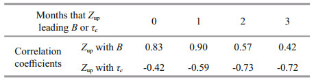
4.3 Interpretation of monthly variability of Zup 4.3.1 Qualitative analysisBased on the relationships of Zup with B and τc, we examine the correlation of Zup to B and τc. The results indicate that Zup has positive correlation with B and negative correlation with τc. Zup presents the best correlation with one-month-advanced B and twomonth-advanced τc, with the correlation coefficient being 0.90 and -0.73 (Table 1), respectively. Accordingly, we conduct a comparative analysis of odd-monthly Zup (January to November, Fig. 3a–f) with even-monthly B (December to the following October, Fig. 5a–f) and odd-monthly τc (November to the following September, Fig. 5g–l).

|
| Figure 5 Climatologically monthly means of the buoyancy flux in even months (a to f is December to the following October) and τc in odd months (g to l is November to the following September) |
On the continental shelf break of the northern SCS, B reaches a positive maximum in December (Fig. 5a) and τc demonstrates a larger negative value in November (Fig. 5g), causing the deepest Zup in January (Fig. 3a). As for the two shallower centers northwest of the Luzon Island and the Kalimantan Island, they are mainly resulted from the largest positive τc and both the negative B and positive τc, respectively.
In February (Fig. 5b), B is smaller than that in December, with a negative value in most areas, so that Zupin March (Fig. 3b) is shallower than that in January. Meanwhile, the two shallower centers of Zup become shallower due to the positive τc (Fig. 5h).
In May, Zup (Fig. 3c) is the shallowest throughout the whole year, mainly owing to the larger negative B in April (Fig. 5c), which plays a dominant role in comparison with τc because of the small |τc| (Fig. 5i).
In July and September, Zup (Fig. 3d, e) in the northwestern SCS is shallower than that in the southeastern SCS. This is because B in the northeastern SCS is smaller than that in the southeastern SCS in June and August (Fig. 5d, e), while τc is positive in the northwestern SCS and larger negative in the southeastern SCS in May and July (Fig. 5j, k).
In October, positive B (Fig. 5f) in the northernmost study region results in the deeper Zup in November (Fig. 3f). In the region between the northwest of the Kalimantan Island and the west of the Luzon Island, τc is positive and a little less than zero (Fig. 5l) on either side of that region. All of these values lead to the fact that Zup in the northern and southeastern SCS is deeper than that in the other areas (Fig. 3f).
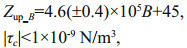
4.3.2 Quantitative interpretationFrom the above qualitative analyses, the buoyancy flux and the wind stress curl can well account for the monthly variability of Zup. In order to analyze the influence level of the buoyancy flux and the wind stress curl on Zup, we explore the relationships of Zup to the buoyancy flux or the wind stress curl without considering the wind stress curl (|τc| < 1×10⁻⁹ N/m3, close to zero) or the buoyancy flux (|B| < 1×10⁻⁷kg/(m·s3), close to zero), respectively. From the linear regression of their results (Fig. 6), it is evident that Zup shows direct proportion to the increasing B, but inverse proportion to the increasing τc. Their empirical relations are given by Eqs.5 and 6, where Zup_B and Zup_τc denote the variations of Zup only resulted from B and τc, respectively. From Eq.5, Zup deepens from 4.2 m to 5.0 m (mean 4.6 m), if B increases by 1×10⁻⁵ kg/(m·s3) without regarding τc. From Eq.6, however, Zup shoals from 1.9 m to 3.1 m (mean 2.5 m), if τc increases by 1×10⁻⁷ N/m3 without taking B into account. In addition, Zup is 45 m without considering either B or τc according to Eqs.5 and 6, resulting in the linear relationship of Zup to B and τc as expressed in Eq.7. Figure 7 describes the odd-monthly mean of Zup resulted from Eq.7. The patterns and values (Fig. 7a–f) are very similar and close to the Zup as shown in Fig. 3a–f, expect in May when Zup resulted from Eq.7 is about 25–30 m (Fig. 7c), which is larger than Zup resulted from SODA (10–15 m) (Fig. 3c) in the northwestern SCS.
 (5)
(5) (6)
(6) (7)
(7)

|
| Figure 6 Linear regression of the buoyancy flux (B) and Zup (a), the wind stress curl (τc) and Zup (b) |

|
| Figure 7 The odd-monthly means (January to November) of Zup resulted from Eq.7 |
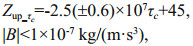
As mentioned above, the factors influencing Zup are the buoyancy flux (B) and the wind stress curl (τc). To further explore the relative importance of B and τc on Zup, we calculate the contribution of B and τc to Zup using Eq.8, where p means the contribution from the buoyancy flux and 100% minus p represents the contribution from the wind stress curl.
As shown in Fig. 8, most of the Zup values are influenced by both the buoyancy flux and the wind stress curl from December to the following February when the wind stress curl dominates the SCS deep basin. The buoyancy flux controls Zup in most regions from April to November (Fig. 8d–k), among which Zup is mainly affected by the buoyancy flux in May and June, while from July to September, Zup in the north of 12°N is mainly influenced by the buoyancy flux with the southern part being dominated by both the buoyancy flux and the wind stress curl.
 (8)
(8)

|
| Figure 8 Distributions of p, Zup is primarily influenced by the wind stress curl when p < 25%, by the buoyancy flux when p > 75%, and by both when p > 25% and p < 75%, (a) to (l) is January to December |
This study examines variability of the upper and lower boundaries of thermocline (Zup and Zlow), its thickness (∆Z) and intensity (Tz) in the SCS, and explores the mechanisms responsible for the monthly variability of Zup. The major results are summarized as follows.
The climatological monthly mean Zup, Zlow, ∆Z and Tz of the SCS are directly or indirectly determined by the vertical temperature GC method from monthly seawater temperature data (1960–2010). The results show that the spatial mean of Zup gradually shoals from February to May and deepens from May to the following January, ∆Z is out of phase with Zup because Zlow remains unchanged all year round.
This study reveals that both the surface buoyancy flux and the wind stress curl play dominant roles in monthly variability of Zup. The variability of surface buoyancy flux (B) resulting from net heat and fresh water flux variations can lead to mix the surface water and change the thickness of the mixed layer, so as to affect the depth of thermocline. The wind stress curl (τc) has the ability to influence Zup through generating upwelling or downwelling. In order to explore how B and τc quantitatively affect Zup, we investigate the monthly B based on the heat flux and precipitation data from NCEP, the evaporation data provided by the Woods Hole Oceanographic Institution, and the τc according to wind stress data from SODA. The results reveal that Zup shows the best correlation to onemonth-advanced B and two-month-advanced τc.
We have analyzed the effects of B and τc on Zup and obtained the regression equation:Zup=4.6(±0.4)×105B– 2.5(±0.6)×107τc+45, which means that Zup has positive correlation with B and negative correlation with τc. Zup deepens from 4.2 m to 5.0 m (mean 4.6 m) when B increases by 1×10⁻⁵ kg/(m·s3) without considering τc, and shoals from 1.9 m to 3.1 m (mean 2.5 m) when τc increases by 1×10⁻⁷ N/m3 regardless of B. The relative importance of the buoyancy flux and the wind stress curl to Zup is also examined, indicating that Zup is mainly controlled by the buoyancy flux throughout the whole year.
Although the Eq.7, resulting from a linear method, can quantitatively account for the influence of B and τc on Zup, there are still some points remaining for discussion. Before using a linear method, the grid points of Zup and B, Zup and τc in the SCS must be the same. Zup and τc which are calculated from SODA products with a 0.5°×0.5° horizontal resolution have the same grid points, but B which is calculated from NCEP (1.875°×1.875°), NOAA (2.5°×2.5°) and WHOI (1°×1°) products has a much fewer grid points than Zup. Therefore, we use the 2-D interpolation method to make B a 0.5°×0.5° horizontal resolution before analyzing the relationship between B and Zup. This may have distorted the Eq.7 somewhat because some grid points of B are from interpolation which could not represent the observations. Moreover, the wind stress (not the wind stress curl) on the sea surface can generate and maintain turbulence to the upper ocean, which would also influence the depth of mixed layer and thermocline. We will take into account the influence of wind stress on Zup in our next step.
6 ACKNOWLEDGEMENTWe thank professor John Hodgkiss of the University of Hong Kong for his help with English.
| Carton J A, Chepurin G, Cao X H, Giese B, 2000a. A simple ocean data assimilation analysis of the global upper ocean 1950-95. Part Ⅰ:methodology. J. Phys. Oceanogr., 30(2): 294–309. Doi: 10.1175/1520-0485(2000)030<0294:ASODAA>2.0.CO;2 |
| Carton J A, Chepurin G, Cao X H, 2000b. A simple ocean data assimilation analysis of the global upper ocean 1950-95.Part Ⅱ:results. J. Phys. Oceanogr., 30(2): 311–326. Doi: 10.1175/1520-0485(2000)030<0311:ASODAA>2.0.CO;2 |
| Carton J A, Giese B S, Grodsky S A, 2005. Sea level rise and the warming of the oceans in the Simple Ocean Data Assimilation (SODA) ocean reanalysis. J. Geophys. Res., 110(C9): C09006. |
| Carton J A, Giese B S, 2008. A reanalysis of ocean climate using Simple Ocean Data Assimilation (SODA). Mon.Wea. Rev., 136(8): 2 999–3 017. |
| Chen M Y, Xie P P, Janowiak J E, Arkin P A, 2002. Global land precipitation:a 50-yr monthly analysis based on gauge observations. J. Hydrometeorol., 3(3): 249–266. |
| China State Bureau of Technical Supervision (CSBTS). 2008. GB/T 12763. 7-2007 The specifications for oceanographic survey-Part 7: exchange of oceanographic survey data. China Standards Press, Beijing. (in Chinese) |
| Fang X J, Wang C X, Xu J J. 2013. Seasenal and interannual variations of the thermocline depth in the South China Sea. Trans. Oceanol. Limnol., (3): 45-55. (in Chinese with English abstract) http://en.cnki.com.cn/Article_en/CJFDTOTAL-HYFB201303006.htm |
| Fofonoff P, Millard Jr R C. 1983. Algorithms for computation of fundamental properties of seawater. UNESCO Tech. Papers in Marine Science 44, UNESCO. 53p. |
| Ge R F, Qiao F L, Yu F, Jiang Z X, Guo J S. 2003. A method for calculating thermocline characteristic elements in shelf sea area-Quasi-step function approximation method. Adv. Mar. Sci., 21(4): 393-400. (in Chinese with English abstract) http://europepmc.org/abstract/CBA/552627 |
| Giese B S, Ray S, 2011. El Niño variability in simple ocean data assimilation (SODA), 1871-2008. J. Geophys. Res., 116(C2): C02024. |
| Gill A E, 1982. Atmosphere-Ocean Dynamics. Academic Press, San Diego, USA. |
| Hao J J, Chen Y L, Wang F, Lin P F, 2012. Seasonal thermocline in the China Seas and northwestern Pacific Ocean. J.Geophys. Res, 117(C2): C02022. |
| Hao J J, Chen Y L, Wang F. 2008. A study of thermocline calculations in the China Sea. Mar. Sci., 32(12): 17-24. (in Chinese with English abstract) http://en.cnki.com.cn/Article_en/CJFDTOTAL-HYKX200812005.htm |
| Kalnay E, Kanamitsu M, Kistler R, Collins W, Deaven D, Gandin L, Iredell M, Saha S, White G, Woollen J, Zhu Y, Leetmaa A, Reynolds B, Chelliah M, Ebisuzaki W, Higgins W, Janowiak J, Mo K C, Ropelewski C, Wang J, Jenne R, Joseph D, 1996. The NCEP/NCAR 40-year reanalysis project. Bull. Amer. Meteor. Soc., 77(3): 437–472. |
| Lan J, Bao Y, Yu F, Sun S W. 2006. Seasonal variabilities of the circulation and thermocline depth in the South China Sea deep water basin. Adv. Mar. Sci., 24(4): 436-445. (in Chinese with English abstract) http://en.cnki.com.cn/article_en/cjfdtotal-hbhh200604003.htm |
| Liu Q Y, Jia Y L, Liu P H, Wang Q, Chu P C, 2001. Seasonal and intraseasonal thermocline variability in the central South China Sea. Geophys. Res. Lett., 28(23): 4 467–4 470. |
| Liu Q Y, Yang H J, Wang Q, 2000. Dynamic characteristics of seasonal thermocline in the deep sea region of the South China Sea. Chin. J. Oceanol. Limnol., 18(2): 104–109. |
| Lozovatsky I, Figueroa M, Roget E, Fernando H J S, Shapovalov S, 2005. Observations and scaling of the upper mixed layer in the North Atlantic. J. Geophys. Res., 110(C5): C05013. |
| McDougall T J, 1987. Neutral surfaces. J. Phys. Oceanogr., 17(11): 1 950–1 964. |
| Schmitt R W, Bogden P S, Dorman C E, 1989. Evaporation minus precipitation and density fluxes for the North Atlantic. J. Phys. Oceanogr., 19(9): 1 208–1 221. |
| Yu L S, Jin X Z, Weller R A. 2008. Multidecade global flux datasets from the objectively analyzed air-sea fluxes(OAFlux) project: latent and sensible heat fluxes, ocean evaporation, and related surface meteorological variables. Woods Hole Oceanographic Institution, OAFlux Project Technical Report. OA-2008-01, Woods Hole, Massachusetts, USA. 64p. |
| Zhou F X, Gao R Z, 2001. Intraseasonal variability of the subsurface temperature observed in the South China Sea(SCS). Chin. Sci. Bull., 47(4): 337–342. |