 2018, Vol. 36
Institute of Oceanology, Chinese Academy of Sciences
Article Information
- KONG Xianyu(孔宪喻), CHE Xiaowei(车潇炜), SU Rongguo(苏荣国), ZHANG Chuansong(张传松), YAO Qingzhen(姚庆祯), SHI Xiaoyong(石晓勇)
- A new technique for rapid assessment of eutrophication status of coastal waters using a support vector machine
- Chinese Journal of Oceanology and Limnology, 36(2): 249-262
- http://dx.doi.org/10.1007/s00343-017-6224-0
Article History
- Received Sep. 19, 2016
- accepted in principle Dec. 12, 2016
- accepted for publication Jan. 4, 2017


Eutrophication is defined as "the enrichment of water by nutrients, especially compounds of nitrogen (N) and/or phosphorus (P) causing an accelerated growth of algae and higher forms of plant life to produce an undesirable disturbance to the balance of organisms present in the water and to the quality of the water concerned" (Ferreira et al., 2010). It often brings about the reduction in light transparency, depletion of dissolved oxygen, the growth of toxic algal blooms and a loss of biodiversity (Hartnett and Nash, 2004; Takaara et al., 2010; Carraro et al., 2012; Rabalais et al., 2014; Tekile et al., 2015; Stefani et al., 2016). In recent decades, it has an increasing tendency toward the eutrophication phenomenon in the coastal and offshore areas due to the stress exerted on the marine environment by terrestrial sources, including industrial activities, agriculture production, transport, energy production, fishing and tourism (Crossland et al., 2005). Eutrophication has aroused a major concern in marine environment protection worldwide due to the serious threats on the aquatic ecosystem and public health (Xue and Landis, 2010; Howarth et al., 2011). Therefore, evaluation of eutrophication is indispensable for regular marine health management and implementation of eutrophication monitoring PROGRAMS that help to understand the variations in marine water quality.
However, some procedures of data collection and analysis for the assessment of eutrophication, such as nutrients, BOD and COD, are usually be determined in a laboratory and usually time-consuming, costly and strenuous, which may not sufficiently facilitate real-time and on-line evaluation and monitoring of the eutrophication of coastal and offshore areas. In fact, the multidimensional property of marine eutrophication means that no single variable can represent the eutrophication status (Cabrita et al., 2015). Although a wide range of physical, chemical, and biological variables contributes to the understanding of coastal marine eutrophication processes, some parameters are highly correlated, undoubtedly, are not all necessary for the development of the eutrophication assessment method (Ignatiades et al., 1985; Primpas and Karydis, 2010). Therefore, the application of several easily measured water quality parameters might have the same effect on assessment of trophic status, and would also facilitate the rapid assessment of eutrophication and implement the real-time monitoring of eutrophication. Chl-a is often considered to be an important and responsive variable that is closely related to water eutrophication (Gibson et al., 2000; Bricker et al., 2008; Fu et al., 2016). Dissolved oxygen is an essential environmental condition for the production of biodegradable organic matter and algal growth and has a significant influence on eutrophication (Rixen et al., 2010; Li et al., 2015; Yan et al., 2016). Turbidity, the cumulative result of total suspended matter and phytoplankton in water environment, is another variable that is strongly related to eutrophication (France and Peters, 1995; Song et al., 2012; Jones et al., 2015). These three variables, easily measured in the field by a multiparameter water quality probe, are most often used for characterizing eutrophication. Many opinions have been stated in the previous studies concerning the use of biological or physicochemical variables for eutrophication assessment. For example, Fernándeza et al. (2014) modeled eutrophication and risk prevention in a reservoir in the Northwest of Spain from biological and physico-chemical parameters (turbidity, DO, temperature, TN, TP, Chlorococcales, and so on) by using multivariate adaptive regression spline analysis. Kuo et al. (2007) used an artificial neural network to relate the key factors that influence a number of water quality indicators, such as DO, Chl-a, TP, and the secchi disk depth, for reservoir eutrophication prediction in a reservoir in central Taiwan.
Currently, multivariate statistical methods are regarded as powerful tools to evaluate eutrophication status because they can combine eutrophic impacts with different aspects of the marine environment. For example, principal component analysis (PCA) has been used to determine the major variables that affect eutrophication processes (Lundberg et al., 2009; Primpas and Karydis, 2010); cluster analysis (CA) has been used to classify different variations into the proper eutrophication status (Stefanou et al., 2000; Primpas et al., 2008); discriminant factor analysis (DFA) has been used to identify variables that can differentiate sampling sites and to group them according to their eutrophication conditions (Tsirtsis and Karydis, 1999; Pinto et al., 2012); and the artificial neural network (ANN) mode has been used in eutrophication assessment due to its simplicity and relatively good fitting output (Jiang et al., 2006; Kuo et al., 2007).
Support vector machine (SVM) has been considered as one most promising approach for evaluating the multidimensional property of marine eutrophication by reflecting the nonlinearity between responsive indicator and environmental factors using structural risk minimization principle and possessing the wellknown ability of being universal approximators of any multivariate function to any desired degree of accuracy (Liu et al., 2016b). In particular, SVM maintains steady performance regardless of input dimensionality and correctly determines the global optimum during the classification process and can avoid overfitting output with better generalization performance (Gokcen and Peng, 2002; Liu and Zhou, 2015). SVM based on machine learning theory is a powerful data classification method that has been applied in predicting values from a wide variety of environmental fields: identification of phytoplankton (Ribeiro and Torgo, 2008), forecast of turbidity (García Nieto et al., 2014), study of water properties (Vilán Vilán et al., 2013), prediction of chlorophyll a concentration (Park et al., 2015), analysis of water level fluctuations (Kisi et al., 2015), and so on. The grid search (GS) algorithm is simple and straightforward to determine the optimize parameter values for the SVM approach classifier (Gao and Hou, 2016). The grid search (GS) algorithm uses grid computing for search processes that provides grid services and information to obtain best interoperability (Bashir et al., 2016). It outperforms both in terms of classification accuracy and computation efficiency. Particularly, when the optimized parameters are many or with great ranges, the grid search (GS) is recommended (Sajan et al., 2015). The effect of the input variables on the degree of eutrophication was assessed by path analysis, which involves standard, multiple, and linear regression techniques to estimate path coefficients and distinguishes causation and interrelation between variables into both direct and indirect effects (Li, 1975; Chesterton et al., 1989). Thus, this study aims to develop a rapid and low-cost method for evaluating the eutrophication status of coastal and offshore waters in the Yellow Sea and East China Sea by SVM in combination with the GS approach, utilizing three easy-to-measure parameters (turbidity, chlorophyll a and dissolved oxygen).
2 MATERIAL AND METHOD 2.1 The study areaAs shown in Fig. 1, a total of 132 sampling sites were chosen in the Yellow Sea and the East China Sea. 294 water samples were collected from 64 sampling sites in July 2013, 132 water samples were collected from 32 sampling sites in November 2013, and 191 water samples were collected from 36 sampling sites in June 2014.

|
| Figure 1 Map of the sampling sites in the Yellow Sea and East China Sea |
The study area (25°50′14.4″S, 120°56′30.012″E to 39°24′49.572″S, 126°51′0.36″E) is a combination of two major marginal seas in the northwest Pacific Ocean, the Yellow Sea (YS) and the East China Sea (ECS). They are topographically connected, but divided subjectively by a line from the mouth of the Changjiang (Yangtze) River to the Cheju Island. The YS, representing a typical shallow marginal sea, is situated between the Korean Peninsula and the mainland China. The ECS, one of the largest marginal seas in the world, is bounded on the west by mainland China and on the east by Kuroshio (Ning et al., 2011). This area is mainly affected by a large range of current systems including the Changjiang Dilute Water, the YS Warm Current, the YS Cold Water Mass, the China Coastal Currents, the Taiwan Warm Current and the Kuroshio Current (Yuan et al., 2008; Yang et al., 2015). The Changjiang River is one of the largest rivers in the world and supplies a large freshwater discharge for adjacent sea regions which obviously changes from the different seasons (Zheng et al., 2015; Pang et al., 2016). Changjiang Diluted Water is divided into two branches when it outflows from the estuary region: one branch spreads to east of the Cheju Island and the other one extends southward along the seashore of Zhejiang Province (Zhu et al., 2011; Sun et al., 2015). The YS and ECS are highly biologically active areas with complicated hydrological variations and are strongly influenced by land-ocean interactions (Shi and Wang, 2012). In recent decades, as a result of high population densities, discharge of domestic and industrial waste, and extensive use of chemical fertilizers, the Changjiang River estuary and adjacent coastal waters have received a high amount of terrestrial nutrients input, consequently, eutrophication has become increasingly serious in these regions (Yuan et al., 2008; Gao et al., 2010; Chen et al., 2016).
2.2 Data collection and analysisThe dataset used was from 595 samples collected in the Yellow Sea and the East China Sea at standard depths, i.e., at the surface; at 10, 20, and 30 m below the surface; and at the bottom, which was determined by the depth of the water. The turbidity and DO concentrations were measured by a CTD multiparameter probe calibrated before the survey. Water samples for the determination of the Chl-a, TN, and TP concentrations were all collected using Niskin bottles mounted on a Seabird CTD Rosette. Water samples for the determination of the TN and TP concentrations were stored in 150-mL acid-cleaned plastic bottles at 4℃ in the field until transport to the laboratory. Samples (500 mL–2 L) for determining Chl-a were filtered through 25-mm glass fiber filters (Whatman GF/F, 0.7-μm pore size) under low vacuum (< 0.3 kPa) and dim light to prevent the degradation of pigments. Measurements of the concentrations of Chl-a, TN, and TP were conducted in the laboratory and finished within two weeks after the cruise. Prior to analysis, all samples were initially warmed to room temperature, after which TN and TP were determined using unfiltered aliquots of samples according to the Valderrama method (Koroleff, 1983a, b). Chl-a was extracted from the filters with 10 mL of acetone (90%) and kept in the dark for 2 h at 4℃. The filter debris was shaped into pellets using a hand-cranked centrifuge, after which the absorbance of the supernatant was measured using a Shimadzu 2550 UV-Vis spectrophotometer calibrated using a blank solution of 90% acetone. The Chl-a concentrations were calculated using the equations of Jeffrey and Humphrey (1975).
2.3 Trophic index (TRIX)The multimetric trophic index TRIX, based on several biological, chemical, and physical parameters, offers a suitable and acceptable method for evaluating coastal eutrophication. It was chosen as an assessment reference for coastal eutrophication in this research. The following formula was used to calculate the coastal eutrophication levels (Vollenweider et al., 1998):
 (1)
(1)where Chl-a=chlorophyll a concentration in μg/L, aD%O=oxygen as an absolute percentage deviation from saturation, TN=total nitrogen in μg/L, TP=total phosphorus in μg/L. The parameters k=1.5 and m=1.2 were ratio coefficients that were selected to define the lower bound value of the trophic index TRIX. The physical significances of the values are presented in Table 1 (Penna et al., 2004).
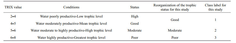
The trophic status index (TRIX) is a linear combination of the logarithms of four variables, allowing the key indicators to be synthesized into a simple numeric expression to make information available over a large array of spatial and temporal trophic status. It aggregates the main cause-effect variables of eutrophication including pressure response, biological response, and environmental disturbance (Pettine et al., 2007; Primpas and Karydis, 2011) and provides useful metrics for the assessment of the trophic status of coastal waters (Cabrita et al., 2015). TRIX has been used for assessing eutrophication in the Black Sea (Moncheva et al., 2002; Parkhomenko et al., 2003), the Caspian Sea (Nasrollahzadeh et al., 2008; Shahrban and Etemad-Shahidi, 2010), the Adriatic sea (Vollenweider et al., 1998; Giovanardi and Vollenweider, 2004; Lušić et al., 2008; Mozetič et al., 2008), and the Baltic Sea (Pettine et al., 2007; Primpas and Karydis, 2011). Only 10 samples were evaluated in this study, which scaled as follows: 2 < TRIX < 4. Thus, the 'high' and 'good' status of the original TRIX was redefined as a 'good' status, and the samples of the dataset were then re-assigned a categorical class label based on the TRIX values: 2 < TRIX < 5=good (class 1), 5≤TRIX < 6=moderate (class 2) and 6≤TRIX < 8=poor (class 3).
2.4 Statistical analysesIn this study, statistical analyses (standard deviations, coefficients of variation, correlation analyses, normal analyses (kurtosis and skewness analyses)) were performed with SPSS 16.0 software. Correlation analyses were used to examine the relationships between the variables. The correlation matrices of all variables are based on the Pearson correlation coefficient, and the significance levels were 0.01 (**) and 0.05 (*). Variables in most statistical approaches are required to conform to a normal distribution; thus, the distribution of each variable was examined by analyzing kurtosis and skewness before support vector machine analyses (Lattin et al., 2003; Papatheodorou et al., 2006).
2.5 Theoretical background for the SVM methodSVM is a powerful new machine learn tool for classification and regression (Taboada et al., 2007; García Nieto et al., 2015). A SVM provides a nonlinear estimation by mapping the input data into a higherdimensional feature space. It uses a set of original data, called support vectors, to establish the optimal hyperplane (HosseinAbadi et al., 2014). The basic idea of SVM can be summarized as follows:
The given training sample is S={(xi, yi), i=1, …, n}, where xi indicates the input vector, yi represents the corresponding desired output vector, n is the number of the training samples. A separating hyperplane, which follows, is constructed in the feature space:
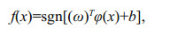 (2)
(2)where ω is the weight parameter that adjusts the construction of the feature hyperplane; φ(·) represents the input data that are mapped into the highdimensional feature space; b is a bias that controls the threshold of margins between the support vectors and the optimized hyperplane. SVM solves the classification problem by finding a hyperplane (ω)Tφ(x)+b=0 (Liu et al., 2016b; Shen et al., 2016).
To map the input data into the N-dimensional space, SVM uses a kernel function. A kernel function allows non-linear data processing via a linear algorithm in the SVM model. Due to the radial basis kernel function (RBF) with simple modality, good smoothness, high learning ability, and easy analyticity, RBF are widely applied to classify data with various samples or dimensions (Liu and Zhou, 2015). Thus, RBF was proposed for as an ideal classification kernel function to construct the SVM model in this study. In the construction of the SVM model, the training dataset was randomly divided into n equal subsets. One subset was employed once as a validation dataset, whereas the other n–1 subsets were grouped into a new training dataset. Cross-validation was the standard technique to find the actual accuracy rates for the analyzed data (Picard and Cook, 1984). The average accuracy of the n validation datasets was regarded as an estimator for the accuracy of the method. In consequence, the combination of optimize parameters with the best performance was chosen (García Nieto et al., 2016). Meanwhile, the grid search (GS) technique was employed to obtain the optimal penalty parameter (C) and kernel function parameter (γ). These must be selected accurately because they determine the structure of the highdimensional feature space and the complexity of the final solution (Park et al., 2015; Sajan et al., 2015).
In this study, a SVM with RBF functions and the GS approach were employed to develop the assessment model for the eutrophication of coastal waters. Figure 2 shows the technical flowchart of the SVM model development. The TRIX classification results were used as target variables, while three variables, turbidity, Chl-a and DO, were used as input variables. The 595 samples were randomly divided into two datasets, i.e., 300 samples in the training dataset and 295 samples in the validation dataset.

|
| Figure 2 Flowchart of the SVM optimization procedure All the SVM algorithms were performed with Matlab 2012. |
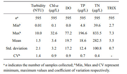
The descriptive statistics for the data are shown in Table 2. The coefficients of variation (C.V.) for Chl-a and DO were both 0.9 and that for turbidity was 1.4. The higher C.V. for turbidity may be because the studied area covered offshore stations with lower turbidity.
|
Kurtosis and skewness analyses demonstrated that DO, turbidity, and Chl-a were almost positively skewed. However, after log transformation of these parameters, all skewness and kurtosis values were significantly reduced, with ranges -1.315–0.202 and -0.012–3.600, respectively. Therefore, all of the aforementioned variables were log transformed prior to SVM analysis.
3.2 Eutrophication status of the Yellow Sea and the East China SeaTable 3 shows the mean, standard error, and ranges of turbidity, Chl-a, DO, TP, and TN of the YS and the ECS. The samples from summer and autumn in the Yellow Sea and the East China Sea show obviously different characteristics of the eutrophication status. TP and TN showed wider ranges in summer than in autumn, suggesting that the larger freshwater input and higher primary production led to a greater trophic status variation in summer (http://www.cjw.gov.cn; Yamaguchi et al., 2013). Large amounts of freshwater discharge from the Changjiang River supply an abundance of nutrients to the Yellow Sea and East China Seas during the summer and intermediate levels of freshwater discharge occur in autumn (Zhu et al., 2009; Yamaguchi et al., 2013; Liu et al., 2016a). The DO values showed an apparent seasonal variation, with higher average values occurring in autumn (7.2±0.10 mg/L) and lower average DO values (5.9±0.07 mg/L) in summer (Table 3). The average DO concentration in autumn was higher than in summer, which was possibly due to the strong vertical eddy mixing in autumn (Wei et al., 2010; Li et al., 2015). Turbidity varied within the range 0.01-9.6 NTU in summer and 0.4-10.0 NTU in autumn (Table 3). Higher concentrations of suspended particulate matter might be due to the resuspension of seabed sediments as a result of the vigorous water mixing that occurred during autumn (Liu et al., 2016a). The average Chl-a concentration in summer was higher than in autumn because of high primary production and low SPM concentration (Gong et al., 2003).

|
Figure 3 shows the spatial distributions of TP, TN, and TRIX in the surface layer in the Yellow Sea and the East China Sea. The highest values of TP, TN, and TRIX index were observed around the Changjiang estuary. This region was characterized by low salinity and relatively high nutrient concentrations. The highest values of the TN, TP and TRIX index in this region might be attributed to freshwater discharges from the Changjiang River, because there are over 13 tributaries flowing into the Changjiang River. Base on the topographic feature of the Chongming Island, the Changjiang estuary is mainly separated into the North Branch and the South Branch. The North Branch receives approximately 5% of the estuarine inputs, whereas the South Branch covers the most flow of the estuary and accounts for more than 95% of the estuarine runoff (Li et al., 2012). The Northern Yellow Sea (NYS) and nearshore area also had higher TP, TN, and TRIX values (Fig. 3a–c) indicating the effects of Bohai Sea and coastal terrestrial inputs from the Yellow Sea Coastal Current and the East China Sea Coastal Current. There is a large amount of water flowing into the NYS from Bohai Sea. Bohai Sea is a semi-enclosed inland sea of China that receives plenty of sediment supply and freshwater discharge from surrounding rivers (Liu, 2015). Influenced by terrigenous inputs, Bohai Sea receives plenty of nutrients (Song et al., 2016). The agricultural runoff, industrial pollution and domestic sewage from the coastal provinces are often transported to the Yellow Sea Coastal Current and the East China Sea Coastal Current by local rivers (Gao et al., 2010; Zhang et al., 2010). Anthropogenic sources could increase the trophic status of the nearshore area.

|
| Figure 3 Distributions of TP, TN, and TRIX in the surface layer in November 2013 (a, b, c) and in July 2013 (d, e, f) in the Yellow Sea and East China Sea |
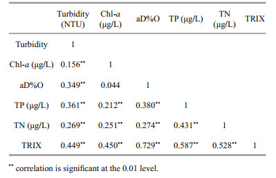
The association between variables was studied by correlation analysis. The DO was significantly correlated with TP (R=0.274, P < 0.01), TN (R=0.380, P < 0.01), and turbidity (R=0.349, P < 0.01). DO, the main factor influencing the nutrient cycle and the release of sediments into the overlying water under certain environmental conditions, has been investigated in many previous studies (Kim et al., 2004; Zhang et al., 2014). Chl-a showed positive correlations with TN (R=0.251, P < 0.01) and TP (R= 0.212, P < 0.01). Nitrogen (N) and phosphorus (P) commonly determine the growth of algae. Excessive nutrients and energy resources often result in nuisance algal blooms (Busse et al., 2006; Liu et al., 2010). Recent studies indicate that Chl-a could be used to predict TN and TP in estuaries and nearshore coastal waters (Meeuwig et al., 2000; Hoyer et al., 2002). Chl-a also exhibited a significant relationship with turbidity (R=0.156, P < 0.01). The growth of biomass in eutrophic status contributes to turbidity, whereas high turbidity might reduce light penetration which impairs the photosynthesis of aquatic algae and vegetation and then affects the eutrophication process (Nicholls et al., 2003). Table 4 shows that turbidity was significantly correlated with TP and TN. Total suspended matter (TSM) usually acts as a carrier for nutrient loading (France and Peters, 1995; Viviano et al., 2014). A few studies have been performed to assess the interrelations among the various parameters related to eutrophication. Xu et al. (2015) developed Support Vector Regression model for the prediction of the TN, TP and Chl-a concentrations affecting Chaohu lake eutrophication using six environment parameters (DO, temperature, pH, flow velocity, disturbance, and experiment time), and their results demonstrated that high correlation coefficients for Chl-a, TN and TP (0.993, 0.996 and 0.976, respectively) have be obtained from the proposed model. Hur and Cho (2012) developed a real-time monitoring tool for the prediction of the BOD, COD, and TN concentrations in a typical urban river using PARAFAC-EEM and UV-Vis absorption indices and demonstrated an enhancement in the estimation capability, with Spearman's rho values of 0.948, 0.977, and 0.984, respectively. Because there were important correlations between the input variables and the nutrients TP and TN, and the output variable TRIX, comprehensive assessments of marine eutrophication levels should consider all of the three input variables.
Pearson correlation coefficients only represent the linear correlation between two variables and may fail to define the complex nature of an ecosystem. A new algorithm must be further explored to reflect the nonlinearity between the responsive variable and the input variables. Therefore, the SVM was employed to predict eutrophication levels using the aforementioned easy-to-measure parameters.
3.4 Model developmentA training dataset was used to determine the parameters and the SVM model was constructed using the GS module. To avoid underfitting and overfitting of the SVM model, an exhaustive 10-fold cross validation technique was used to select the optimal SVM parameters which can simulate as many as possible the real situations so that the model could adapt the new observations (Picard and Cook, 1984; Sajan et al., 2015). The training dataset was randomly divided into 10 equal subsets. Each subset was employed once as a validation dataset, whereas the other 9 subsets were grouped into a new training dataset, and the optimal parameters of the SVM model was found with the grid search (GS) technique (Cristianini and Shawe-Taylor, 2000; Zhang et al., 2016). In this way, all the possible variability of the SVM model has been estimated in order to obtain the optimal parameters that minimize the average error. The results of classification are mainly affected by kernel function parameter (γ) and the penalty parameter (C), which must be carefully determined in the SVM model because the former determines the accuracy of the classification function and the latter controls the tradeoff between the training error and model flatness (Liu et al., 2006; Xu et al., 2015). Since the two parameters C and γ are independent, the GS process can be conducted in parallel. Specifically, a set of candidates are firstly selected for both γ and C. Then each pair of C and γ is evaluated by crossvalidation and the pair with the highest accuracy is determined as the optimal parameters (Gao and Hou, 2016). Figure 4 shows the map of optimization results of the SVM model. Both the penalty parameter C had optimal values of 64 and the kernel function parameter γ was 1. The classification accuracy is the main fitness factor.

|
| Figure 4 Map of optimized SVM parameters obtained by grid search |
Using the optimal parameters mentioned above, 107 input datasets were selected as support vectors. The outcome was a trained SVM classification model. The classification accuracy rate was 88.3% for the cross-validation and 89.3% for the training dataset. These results clearly indicate the consistency between experimental results and model predictions and confirm the validity of the SVC model. The classification decision function is expressed as Eq.3:
 (3)
(3)where x and xi are input vector spaces, ai is Lagrange's multiplier, yi is the class label, and b is a scalar threshold that adjusts the bias of margins between the optimal hyperplane and the support vectors.
3.5 Model validationThe 295 samples of the validation dataset were used to verify the performance of the developed model, and the classification results are presented in Table 5. The overall classification accuracy was 88.5% for the validation dataset. The samples of good, moderate, and poor trophic status were all well classified by the SVM model (91.0%, 90.4%, and 82.0%, respectively). The incorrectly classified samples included 6 samples of good status, 15 samples of moderate status and 13 samples of poor status according to TRIX classification, in which 3 of the 6 good status samples had TRIX values of 4.9 to 5.0, 9 of 15 moderate status samples had TRIX values of 5.0 to 5.1 or 5.9 to 6.0, and 9 of 13 poor status samples had TRIX values of 6.0 to 6.1. Most incorrectly classified samples had TRIX values near the boundaries. These results indicate good agreement between the SVM model and the multimetric trophic index TRIX. Therefore, it is feasible to use SVM as an effective approach to solve the problem of nonlinearities of the eutrophication status.

The SVM is a typical approach of artificial intelligence machine learning as a non-linear solution for classification problems (Vapnik, 1995; Behzad et al., 2009). In particular, SVM accurately defines the global optimum values and can thus avoid over-fitting the output values, resulting in better generalization performance. (Kovačević et al., 2010). Using SVM, we developed an eutrophication prediction method for coastal waters with high prediction accuracy. This methodology was successfully applied to evaluate the eutrophication levels of the Yellow Sea and East China Sea. Pinto et al. (2012) developed a two-level discriminant function analysis model for rapidly assessing the eutrophication risk (high or low) of a river from three easy-to-measure parameters (DO, turbidity, and temperature), providing an approximate 72% prediction accuracy. Comparatively, the method developed by the SVM had a better performance, although it is always necessary to take into account the specificities of each location when used in other waters.
The study periods of summer and autumn in the Yellow Sea and the East China Sea showed significantly different characteristics of eutrophication status and the study area covered most of the coastal and offshore areas in the Yellow Sea and the East China Sea. The model developed here can adapt to the temporal and spatial variation of water quality parameters in the Yellow Sea and the East China Sea. Additionally, it can offer potential cost savings in marine monitoring programs considering that the model only uses three easy-to-measure variables: DO, Chl-a, and turbidity. As such, this is an important finding and its application can help in rapid assessment of coastal and offshore areas.
3.6 Role of key variables in the SVM modelPath analysis is an extension of the regression model, and its path coefficients are often used to assess the relative importance of various direct and indirect causal paths (the input variables) to the dependent variable (Streiner, 2005; Garson, 2008). In this study, path analysis was applied to investigate the importance of input variables DO, Chl-a, and turbidity that influence eutrophication levels, which could indirectly assist in identifying situations that might yield better model performances. Table 6 shows the direct, indirect, and total effects of DO, turbidity, Chla, and ranks the influence of the input variables on the eutrophication level.

|
Among the three input variables, DO had the most significant effect on the evaluated eutrophication levels (Table 6). It is indispensable to the respiratory metabolism of most aquatic organisms and impacts the availability of nutrients and thus influences the productivity of marine ecosystems (García Nieto et al., 2013). DO was the main factor influencing the release of nutrients from the sediments into the overlying water under certain environmental states that could have a strong influence on the eutrophication status and the quality of water (Xie et al., 2003; Kim et al., 2004). The DO levels in water are very complicated and are mostly dependent on the salinity, temperature, depth, degradation of organic matter and the photosynthesis and respiration of phytoplankton (Badran, 2001; Wheeler et al., 2003; Manasrah et al., 2006). Turbidity had the most significant indirect contribution to the trophic state assessment by the SVM model. This is probably partly because turbidity is greatly influenced by the presence of organic and inorganic matter (Pinto et al., 2012). It is often used as an important test for water quality control. Turbidity as a variable is strongly related to eutrophication (Alonso Fernández et al., 2014). Most of the suspended matter has a large impact on the production of phytoplankton, macrophyte and periphyton communities by affecting the availability of light in the marine environment (Waters, 1995; Bilotta and Brazier, 2008). Therefore, turbidity plays a crucial part in determining the light intensity and impacting phytoplankton productivity. Chlorophyll a is a major photosynthetic pigment found in the phytoplankton species and its concentration is often used as an estimator of the productivity of the water body. It is one of the common water quality indicators for the assessment of the eutrophication status of the water environment (Lillesand et al., 1983; Baban, 1996).
In this study, the input variables were restricted to those parameters that were available by a CTD multiparameter probe. However, further research is needed to explore other easily measured variables that may improve the accuracy of SVM model prediction, such as absorption and fluorescence parameters of chromophoric dissolved organic matter (CDOM). CDOM is often coupled with nutrients and plays an important part in the biogeochemistry cycle of nutrients. Absorption and fluorescence measurements could provide information on the concentration and composition of CDOM (Stedmon et al., 2007; Zhang et al., 2011). It is also necessary to validate the SVM model with long-term data that will support the future feasibility of the model.
4 CONCLUSIONUsing the SVM approach, we developed an eutrophication prediction model for coastal and offshore areas in the Yellow Sea and the East China Sea. With the optimized penalty parameter C=64 and the kernel parameter γ=1 obtained in training process, the classification accuracy rates reached 89.3% for the training data, 88.3% for the cross-validation, and 88.5% for the validation dataset. As demonstrated here, the application of only three easy-to-measure variables, DO, Chl-a, and turbidity resulted in the successful application of this model to evaluate TRIX classification in the Yellow Sea and the East China Sea. Thus, the application of the model can assist in the rapid assessment eutrophication of marine conditions and regularly implement marine health management and eutrophication monitoring programs. Additionally, we are confident that the results obtained in this research will be beneficial to enhance future work along similar fields, i.e., to develop other methodologies for assessment of eutrophication. Furthermore, the integrated SVM based classification method and framework might have a large application potential, not only in trophic status evaluation but also in other environmental areas when it is well explored.
| Baban S M J, 1996. Trophic classification and ecosystem checking of lakes using remotely sensed information. Hydrological Sciences Journal, 41(6): 939–957. Doi: 10.1080/02626669609491560 |
| Badran M I, 2001. Dissolved oxygen, chlorophyll a and nutrients:seasonal cycles in waters of the Gulf of Aquaba, Red Sea. Aquat. Ecosyst. Health Manage., 4(2): 139–150. Doi: 10.1080/14634980127711 |
| Bashir M B, Latiff M S B A, Coulibaly Y, Yousif A, 2016. A survey of grid-based searching techniques for large scale distributed data. Journal of Network and Computer Applications, 60: 170–179. Doi: 10.1016/j.jnca.2015.10.010 |
| Behzad M, Asghari K, Eazi M, Palhang M, 2009. Generalization performance of support vector machines and neural networks in runoff modeling. Expert Systems with Applications, 36(4): 7 624–7 629. Doi: 10.1016/j.eswa.2008.09.053 |
| Bilotta G S, Brazier R E, 2008. Understanding the influence of suspended solids on water quality and aquatic biota. Water Res., 42(12): 2 849–2 861. Doi: 10.1016/j.watres.2008.03.018 |
| Bricker S B, Longstaff B, Dennison W, Jones A, Boicourt K, Wicks C, Woerner J, 2008. Effects of nutrient enrichment in the nation's estuaries:a decade of change. Harmful Algae, 8(1): 21–32. Doi: 10.1016/j.hal.2008.08.028 |
| Busse L B, Simpson J C, Cooper S D, 2006. Relationships among nutrients, algae, and land use in urbanized southern California streams. Can. J. Fish. Aquat. Sci., 63(12): 2 621–2 638. Doi: 10.1139/f06-146 |
| Cabrita M T, Silva A, Oliveira P B, Angélico M M, Nogueira M, 2015. Assessing eutrophication in the Portuguese continental exclusive economic zone within the European marine strategy framework directive. Ecological Indicators, 58: 286–299. Doi: 10.1016/j.ecolind.2015.05.044 |
| Carraro E, Guyennon N, Hamilton D, Valsecchi L, Manfredi E C, Viviano G, Salerno F, Tartari G, Copetti D, 2012. Coupling high-resolution measurements to a threedimensional lake model to assess the spatial and temporal dynamics of the cyanobacterium Planktothrix rubescens in a medium-sized lake. Hydrobiologia, 698(1): 77–95. Doi: 10.1007/s10750-012-1096-y |
| Chen Y, Yang G P, Liu L, Zhang P Y, Leng W S, 2016. Sources, behaviors and degradation of dissolved organic matter in the East China Sea. J. Mar. Syst., 155: 84–97. Doi: 10.1016/j.jmarsys.2015.11.005 |
| Chesterton R N, Pfeiffer D U, Morris R S, Tanner C M, 1989. Environmental and behavioural factors affecting the prevalence of foot lameness in New Zealand dairy herds-a case-control study. New Zeal. Vet. J., 37(4): 135–142. Doi: 10.1080/00480169.1989.35587 |
| Cristianini N, Shawe-Taylor J. 2000. An Introduction to Support Vector Machines and Other Kernel-Based Learning Methods. Cambridge University Press, Cambridge. http://dl.acm.org/citation.cfm?id=345662 |
| Crossland C J, Kremer H H, Lindeboom H, Marshall Crossland J I, Le Tissier M D A. 2005. Coastal Fluxes in the Anthropocene. Springer, Berlin. |
| Fernández J R A, Nieto P J G, Muñiz C D, Antón J C Á, 2014. Modeling eutrophication and risk prevention in a reservoir in the Northwest of Spain by using multivariate adaptive regression splines analysis. Ecological Engineering, 68: 80–89. Doi: 10.1016/j.ecoleng.2014.03.094 |
| Ferreira J G, Andersen J H, Borja A, Bricker S B, Camp J, Cardoso da Silva M, Garcés E, Heiskanen A S, Humborg C, Ignatiades L, Lancelot C, Menesguen A, Tett P, Hoepffner N, Claussen U. 2010. Marine Strategy Framework Directive-Task Group 5 Report Eutrophication. JRC Scientific and Technical Reports. Office for Official Publications of the European Communities, Luxembourg. 49p. |
| France R L, Peters R H, 1995. Predictive model of the effects on lake metabolism of decreased airborne litterfall through riparian deforestation. Conserv. Biol., 9(6): 1 578–1 586. Doi: 10.1046/j.1523-1739.1995.09061578.x |
| Fu M Z, Wang Z L, Pu X M, Qu P, Li Y, Wei Q S, Jiang M J, 2016. Response of phytoplankton community to nutrient enrichment in the subsurface chlorophyll maximum in Yellow Sea Cold Water Mass. Acta Ecologica Sinica, 36(1): 39–44. Doi: 10.1016/j.chnaes.2015.09.007 |
| Gao L, Fan D D, Li D J, Cai J G, 2010. Fluorescence characteristics of chromophoric dissolved organic matter in shallow water along the Zhejiang coasts, southeast China. Mar. Environ. Res., 69(3): 187–197. Doi: 10.1016/j.marenvres.2009.10.004 |
| Gao X, Hou J, 2016. An improved SVM integrated GS-PCA fault diagnosis approach of Tennessee Eastman process. Neurocomputing, 174: 906–911. Doi: 10.1016/j.neucom.2015.10.018 |
| García Nieto P J, Alonso Fernández J R, de Cos Juez F J, Sánchez Lasheras F S, Díaz Muñiz C, 2013. Hybrid modelling based on support vector regression with genetic algorithms in forecasting the cyanotoxins presence in the Trasona reservoir (Northern Spain). Environ. Res., 122: 1–10. Doi: 10.1016/j.envres.2013.01.001 |
| García Nieto P J, García-Gonzalo E, Alonso Fernández J R, Díaz Muñiz C, 2014. Hybrid PSO-SVM-based method for long-term forecasting of turbidity in the Nalón river basin:a case study in Northern Spain. Ecological Engineering, 73: 192–200. Doi: 10.1016/j.ecoleng.2014.09.042 |
| García Nieto P J, García-Gonzalo E, Alonso Fernández J R, Díaz Muñiz C, 2016. A hybrid PSO optimized SVMbased model for predicting a successful growth cycle of the Spirulina platensis from raceway experiments data. J. Comput. Appl. Math., 291: 293–303. Doi: 10.1016/j.cam.2015.01.009 |
| García Nieto P J, García-Gonzalo E, Sánchez Lasheras F, de Cos Juez F J, 2015. Hybrid PSO-SVM-based method for forecasting of the remaining useful life for aircraft engines and evaluation of its reliability. Reliab. Eng. Syst. Saf., 138: 219–231. Doi: 10.1016/j.ress.2015.02.001 |
| Garson G D. 2008. Path analysis. from Statnotes: topics in multivariate analysis. Retrieved, 9(5): 2009. |
| Gibson G, Carlson R, Simpson J, Smeltzer E. 2000. Nutrient criteria technical guidance manual: lakes and reservoirs(EPA-822-B-00-001). United States Environment Protection Agency, Washington DC. |
| Giovanardi F, Vollenweider R A, 2004. Trophic conditions of marine coastal waters:experience in applying the Trophic Index TRIX to two areas of the Adriatic and Tyrrhenian seas. J. Limnol., 63(2): 199–218. Doi: 10.4081/jlimnol.2004.199 |
| Gokcen I, Peng J. 2002. Comparing linear discriminant analysis and support vector machines. In: Yakhno T ed. Advances in Information Systems: Lecture Notes in Computer Science, 2457. Springer, Berlin Heidelberg. p. 104-113. |
| Gong G C, Wen Y H, Wang B W, Liu G J, 2003. Seasonal variation of chlorophyll a concentration, primary production and environmental conditions in the subtropical East China Sea. Deep Sea Research Part Ⅱ:Topical Studies in Oceanography, 50(6-7): 1 219–1 236. Doi: 10.1016/S0967-0645(03)00019-5 |
| Hartnett M, Nash S, 2004. Modelling nutrient and chlorophyll_a dynamics in an Irish brackish waterbody. Environ. Modell. Softw., 19(1): 47–56. Doi: 10.1016/S1364-8152(03)00109-9 |
| HosseinAbadi H Z, Amirfattahi R, Nazari B, Mirdamadi H R, Atashipour S A, 2014. GUW-based structural damage detection using WPT statistical features and multiclass SVM. Appl. Acoust., 86: 59–70. Doi: 10.1016/j.apacoust.2014.05.002 |
| Howarth R, Chan F, Conley D J, Garnier J, Doney S C, Marino R, Billen G, 2011. Coupled biogeochemical cycles:eutrophication and hypoxia in temperate estuaries and coastal marine ecosystems. Front. Ecol. Environ., 9(1): 18–26. Doi: 10.1890/100008 |
| Hoyer M V, Frazer T K, Notestein S K, Canfield Jr D E, 2002. Nutrient, chlorophyll, and water clarity relationships in Florida's nearshore coastal waters with comparisons to freshwater lakes. Can. J. Fish. Aquat. Sci., 59(6): 1 024–1 031. Doi: 10.1139/f02-077 |
| Hur J, Cho J, 2012. Prediction of BOD, COD, and total nitrogen concentrations in a typical urban river using a fluorescence excitation-emission matrix with PARAFAC and UV absorption indices. Sensors, 12(1): 972–986. Doi: 10.3390/s120100972 |
| Ignatiades L, Vassiliou A, Karydis M, 1985. A comparison of phytoplankton biomass parameters and their interrelation with nutrients in Saronicos Gulf (Greece). Hydrobiologia, 128(3): 201–206. Doi: 10.1007/BF00006815 |
| Jeffrey S W, Humphrey G F, 1975. New spectrophotometric equations for determining chlorophylls a, b, c1 and c2 in higher plants, algae and natural phytoplankton. Biochem. Physiol. Pflanz., 167: 191–194. Doi: 10.1016/S0015-3796(17)30778-3 |
| Jiang Y P, Xu Z X, Yin H L, 2006. Study on improved BP artificial neural networks in eutrophication assessment of China eastern lakes. J. Hydrodyn. Ser. B., 18(S3): 528–532. |
| Jones S, Carrasco N K, Perissinotto R, 2015. Turbidity effects on the feeding, respiration and mortality of the copepod Pseudodiaptomus stuhlmanni in the St Lucia Estuary, South Africa. Journal of Experimental Marine Biology and Ecology, 469: 63–68. Doi: 10.1016/j.jembe.2015.04.015 |
| Kim L H, Choi E, Gil K I, Stenstrom M K, 2004. Phosphorus release rates from sediments and pollutant characteristics in Han River, Seoul, Korea. Sci. Total Environ., 321(1-3): 115–125. Doi: 10.1016/j.scitotenv.2003.08.018 |
| Kisi O, Shiri J, Karimi S, Shamshirband S, Motamedi S, Petković D, Hashim R, 2015. A survey of water level fluctuation predicting in Urmia Lake using support vector machine with firefly algorithm. Appl. Math. Comput., 270: 731–743. |
| Koroleff F. 1983a. Determination of phosphorus. In: Grasshoff K, Ehrhardt M, Kremling K eds. Methods of Seawater Analysis. Verlag Chemie, Weinheim, Germany. p. 125-139. |
| Koroleff F. 1983b. Total and organic nitrogen. In: Grasshoff K, Ehrhardt M, Kremling K eds. Methods of Seawater Analysis. Verlag Chemie, Weinheim, Germany. p. 162-173. |
| Kovačević M, Bajat B, Gajić B, 2010. Soil type classification and estimation of soil properties using support vector machines. Geoderma, 154(3-4): 340–347. Doi: 10.1016/j.geoderma.2009.11.005 |
| Kuo J T, Hsieh M H, Lung W S, She N, 2007. Using artificial neural network for reservoir eutrophication prediction. Ecol. Model., 200(1-2): 171–177. Doi: 10.1016/j.ecolmodel.2006.06.018 |
| Lattin J M, Carroll J D, Green P E. 2003. Analyzing Multivariate Data. Thomson Brooks/Cole, Pacific Grove, CA. |
| Li B H, Feng C H, Li X, Chen Y X, Niu J F, Shen Z Y, 2012. Spatial distribution and source apportionment of PAHs in surficial sediments of the Yangtze Estuary, China. Mar. Pollut. Bull., 64(3): 636–643. Doi: 10.1016/j.marpolbul.2011.12.005 |
| Li C C. 1975. Introduction, multiple regression and correlation, standardized variables; path coefficients. In: Li C C ed. Path Analysis-A Primer. Pacific Grove, California. p. 75-100. |
| Li H M, Zhang C S, Han X R, Shi X Y, 2015. Changes in concentrations of oxygen, dissolved nitrogen, phosphate, and silicate in the southern Yellow Sea, 1980-2012:sources and seaward gradients. Estuar. Coast. Shelf Sci., 163: 44–55. |
| Lillesand T M, Johnson W L, Deuell R L, Lindstrom O M, Meisner D E, 1983. Use of Landsat data to predict the trophic state of Minnesota lakes. Photogram. Eng. Remote Sensing, 49(2): 219–229. |
| Liu F, Zhou Z G, 2015. A new data classification method based on chaotic particle swarm optimization and least squaresupport vector machine. Chemom. Intell. Lab. Syst., 147: 147–156. Doi: 10.1016/j.chemolab.2015.08.015 |
| Liu S M, Qi X H, Li X N, Ye H R, Wu Y, Ren J L, Zhang J, Xu W Y, 2016a. Nutrient dynamics from the Changjiang(Yangtze River) estuary to the East China Sea. J. Mar.Syst., 154: 15–27. Doi: 10.1016/j.jmarsys.2015.05.010 |
| Liu S M, 2015. Response of nutrient transports to water-sediment regulation events in the Huanghe basin and its impact on the biogeochemistry of the Bohai. J. Mar. Syst., 141: 59–70. Doi: 10.1016/j.jmarsys.2014.08.008 |
| Liu X, Lu W, Jin S, Li Y, Chen N, 2006. Support vector regression applied to materials optimization of sialon ceramics. Chemom. Intell. Lab. Syst., 82(1-2): 8–14. Doi: 10.1016/j.chemolab.2005.08.011 |
| Liu Y, Guo H C, Yang P J, 2010. Exploring the influence of lake water chemistry on chlorophyll a:a multivariate statistical model analysis. Ecol. Model., 221(4): 681–688. Doi: 10.1016/j.ecolmodel.2009.03.010 |
| Liu Y, Wang H F, Zhang H, Liber K, 2016b. A comprehensive support vector machine-based classification model for soil quality assessment. Soil and Tillage Research, 155: 19–26. Doi: 10.1016/j.still.2015.07.006 |
| Lundberg C, Jakobsson B M, Bonsdorff E, 2009. The spreading of eutrophication in the eastern coast of the Gulf of Bothnia, northern Baltic Sea-an analysis in time and space. Estuar. Coast. Shelf Sci., 82(1): 152–160. Doi: 10.1016/j.ecss.2009.01.005 |
| Lušić D V, Peršić V, Horvatić J, Viličić D, Traven L, Đakovac T, Mićović V, 2008. Assessment of nutrient limitation in Rijeka Bay, NE Adriatic Sea, using miniaturized bioassay. Journal of Experimental Marine Biology and Ecology, 358(1): 46–56. Doi: 10.1016/j.jembe.2008.01.012 |
| Manasrah R, Raheed M, Badran M I, 2006. Relationships between water temperature, nutrients and dissolved oxygen in the northern Gulf of Aqaba, Red Sea. Oceanologia, 48(2): 237–253. |
| Meeuwig J J, Kauppila P, Pitkänen H, 2000. Predicting coastal eutrophication in the Baltic:a limnological approach. Can. J. Fish. Aquat. Sci., 57(4): 844–855. Doi: 10.1139/f00-013 |
| Moncheva S, Dontcheva V, Shtereva G, Kamburska L, Malej A, Gorinstein S, 2002. Application of eutrophication indices for assessment of the Bulgarian Black Sea coastal ecosystem ecological quality. Water Sci. Technol., 46(8): 19–28. |
| Mozetič P, Malačič V, Turk V, 2008. A case study of sewage discharge in the shallow coastal area of the Northern Adriatic Sea (Gulf of Trieste). Mar. Ecol., 29(4): 483–494. Doi: 10.1111/mae.2008.29.issue-4 |
| Nasrollahzadeh H S, Din Z B, Foong S Y, Makhlough A, 2008. Trophic status of the Iranian Caspian Sea based on water quality parameters and phytoplankton diversity. Cont.Shelf Res., 28(9): 1 153–1 165. Doi: 10.1016/j.csr.2008.02.015 |
| Nicholls K H, Steedman R J, Carney E C, 2003. Changes in phytoplankton communities following logging in the drainage basins of three boreal forest lakes in northwestern Ontario (Canada), 19912000. Can. J. Fish. Aquat. Sci., 60(1): 43–54. Doi: 10.1139/f03-002 |
| Ning X, Lin C, Su J, Liu C, Hao Q, Le F, 2011. Long-term changes of dissolved oxygen, hypoxia, and the responses of the ecosystems in the East China Sea from 1975 to 1995. J. Oceanogr., 67(1): 59–75. Doi: 10.1007/s10872-011-0006-7 |
| Pang C G, Li K, Hu D X, 2016. Net accumulation of suspended sediment and its seasonal variability dominated by shelf circulation in the Yellow and East China Seas. Mar. Geol., 371: 33–43. Doi: 10.1016/j.margeo.2015.10.017 |
| Papatheodorou G, Demopoulou G, Lambrakis N, 2006. A long-term study of temporal hydrochemical data in a shallow lake using multivariate statistical techniques. Ecol. Model., 193(3-4): 759–776. Doi: 10.1016/j.ecolmodel.2005.09.004 |
| Park Y, Cho K H, Park J, Cha S M, Kim J H, 2015. Development of early-warning protocol for predicting chlorophyll-a concentration using machine learning models in freshwater and estuarine reservoirs, Korea. Sci. Total Environ., 502: 31–41. Doi: 10.1016/j.scitotenv.2014.09.005 |
| Parkhomenko A V, Kuftarkova E A, Subbotin A A, Gubanov V I, 2003. Results of hydrochemical monitoring of Sevastopol Black Sea's offshore waters. J. Coastal Res., 19(4): 907–911. |
| Penna N, Capellacci S, Ricci F, 2004. The influence of the Po River discharge on phytoplankton bloom dynamics along the coastline of Pesaro (Italy) in the Adriatic Sea. Mar.Pollut. Bull., 48(3-4): 321–326. Doi: 10.1016/j.marpolbul.2003.08.007 |
| Pettine M, Casentini B, Fazi S, Giovanardi F, Pagnotta R, 2007. A revisitation of TRIX for trophic status assessment in the light of the European Water Framework Directive:application to Italian coastal waters. Mar. Pollut. Bull., 54(9): 1 413–1 426. Doi: 10.1016/j.marpolbul.2007.05.013 |
| Picard R R, Cook R D, 1984. Cross-validation of regression models. J. Amer. Statist. Assoc., 79(387): 575–583. |
| Pinto U, Maheshwari B, Shrestha S, Morris C, 2012. Modelling eutrophication and microbial risks in peri-urban river systems using discriminant function analysis. Water Res., 46(19): 6 476–6 488. Doi: 10.1016/j.watres.2012.09.025 |
| Primpas I, Karydis M, Tsirtsis G, 2008. Assessment of clustering algorithms in discriminating eutrophic levels in coastal waters. Glob. NEST J., 10(3): 359–365. |
| Primpas I, Karydis M, 2010. Improving statistical distinctness in assessing trophic levels:the development of simulated normal distributions. Environ. Monit. Assess., 169(1-4): 353–365. Doi: 10.1007/s10661-009-1177-1 |
| Primpas I, Karydis M, 2011. Scaling the trophic index (TRIX) in oligotrophic marine environments. Environ. Monit. Assess., 178(1-4): 257–269. Doi: 10.1007/s10661-010-1687-x |
| Rabalais N N, Cai W J, Carstensen J, Conley D, Fry B, Hu X, Quiñones-Rivera Z, Rosenberg R, Slomp C P, Turner R E, Voss M, Wissel B, Zhang J, 2014. Eutrophication-driven deoxygenation in the coastal ocean. Oceanography, 27(1): 172–183. Doi: 10.5670/oceanog |
| Ribeiro R, Torgo L, 2008. A comparative study on predicting algae blooms in Douro River, Portugal. Ecol. Model., 212(1-2): 86–91. Doi: 10.1016/j.ecolmodel.2007.10.018 |
| Rixen T, Baum A, Sepryani H, Pohlmann T, Jose C, Samiaji J, 2010. Dissolved oxygen and its response to eutrophication in a tropical black water river. J. Environ. Manag., 91(8): 1 730–1 737. Doi: 10.1016/j.jenvman.2010.03.009 |
| Sajan K S, Kumar V, Tyagi B, 2015. Genetic algorithm based support vector machine for on-line voltage stability monitoring. Int. J. Elec. Power Energy Syst., 73: 200–208. Doi: 10.1016/j.ijepes.2015.05.002 |
| Shahrban M, Etemad-Shahidi A, 2010. Classification of the Caspian Sea coastal waters based on trophic index and numerical analysis. Environ. Monit. Assess., 164(1-4): 349–356. Doi: 10.1007/s10661-009-0897-6 |
| Shen X J, Mu L, Li Z, Wu H X, Gou J P, Chen X, 2016. Largescale support vector machine classification with redundant data reduction. Neurocomputing, 172: 189–197. Doi: 10.1016/j.neucom.2014.10.102 |
| Shi W, Wang M H, 2012. Satellite views of the Bohai Sea, Yellow Sea, and East China Sea. Prog. Oceanogr., 104: 30–45. Doi: 10.1016/j.pocean.2012.05.001 |
| Song K S, Li L, Li S, Tedesco L, Hall B, Li L H, 2012. Hyperspectral remote sensing of total phosphorus (TP) in three central Indiana water supply reservoirs. Water Air Soil Pollut., 223(4): 1 481–1 502. Doi: 10.1007/s11270-011-0959-6 |
| Song N Q, Wang N, Lu Y, Zhang J R, 2016. Temporal and spatial characteristics of harmful algal blooms in the Bohai Sea during 1952-2014. Cont. Shelf Res., 122: 77–84. Doi: 10.1016/j.csr.2016.04.006 |
| Stedmon C A, Markager S, Tranvik L, Kronberg L, Slätis T, Martinsen W, 2007. Photochemical production of ammonium and transformation of dissolved organic matter in the Baltic Sea. Mar. Chem., 104(3-4): 227–240. Doi: 10.1016/j.marchem.2006.11.005 |
| Stefani F, Salerno F, Copetti D, Rabuffetti D, Guidetti L, Torri G, Naggi A, Iacomini M, Morabito G, Guzzella L, 2016. Endogenous origin of foams in lakes:a long-term analysis for Lake Maggiore (northern Italy). Hydrobiologia, 767(1): 249–265. Doi: 10.1007/s10750-015-2506-8 |
| Stefanou P, Tsirtsis G, Karydis M, 2000. Nutrient scaling for assessing eutrophication:the development of a simulated normal distribution. Ecol. Appl., 10(1): 303–309. Doi: 10.1890/1051-0761(2000)010[0303:NSFAET]2.0.CO;2 |
| Streiner D L, 2005. Finding our way:an introduction to path analysis. Can. J. Psychiatry, 50(2): 115–122. Doi: 10.1177/070674370505000207 |
| Sun S, Zhang F, Li C L, Wang S W, Wang M X, Tao Z C, Wang Y T, Zhang G T, Sun X X, 2015. Breeding places, population dynamics, and distribution of the giant jellyfish Nemopilema nomurai (Scyphozoa:Rhizostomeae) in the Yellow Sea and the East China Sea. Hydrobiologia, 754(1): 59–74. Doi: 10.1007/s10750-015-2266-5 |
| Taboada J, Matías J M, Ordóñez C, García P J, 2007. Creating a quality map of a slate deposit using support vector machines. J. Comput. Appl. Math., 204(1): 84–94. Doi: 10.1016/j.cam.2006.04.030 |
| Takaara T, Sano D, Masago Y, Omura T, 2010. Surface-retained organic matter of Microcystis aeruginosa inhibiting coagulation with polyaluminum chloride in drinking water treatment. Water Res., 44(13): 3 781–3 786. Doi: 10.1016/j.watres.2010.04.030 |
| Tekile A, Kim I, Kim J, 2015. Mini-review on river eutrophication and bottom improvement techniques, with special emphasis on the Nakdong River. J. Environ. Sci., 30: 113–121. Doi: 10.1016/j.jes.2014.10.014 |
| Tsirtsis G, Karydis M. 1999. Application of discriminant analysis for water quality assessment in the Aegean. In: Proceedings of the 6th Conference on Environmental Science and Technology. Univ. of the Aegean, Samos, Greece. |
| Vapnik V N. 1995. The Nature of Statistical Learning Theory. Springer, New York. |
| Vilán Vilán J A, Alonso Fernández J R, García Nieto P J, Sánchez Lasheras F, de Cos Juez F J, Díaz Muñiz C, 2013. Support vector machines and multilayer perceptron networks used to evaluate the cyanotoxins presence from experimental cyanobacteria concentrations in the Trasona reservoir (Northern Spain). Water. Resour. Manage., 27: 3 457–3 476. Doi: 10.1007/s11269-013-0358-4 |
| Viviano G, Salerno F, Manfredi E C, Polesello S, Valsecchi S, Tartari G, 2014. Surrogate measures for providing high frequency estimates of total phosphorus concentrations in urban watersheds. Water Res., 64: 265–277. Doi: 10.1016/j.watres.2014.07.009 |
| Vollenweider R A, Giovanardi F, Montanari G, Rinaldi A, 1998. Characterization of the trophic conditions of marine coastal waters with special reference to the NW Adriatic Sea:proposal for a trophic scale, turbidity and generalized water quality index. Environmetrics, 9(3): 329–357. Doi: 10.1002/(ISSN)1099-095X |
| Waters T F. 1995. Sediment in Streams: Sources, Biological Effects, and Control. American Fisheries Society, Bethesda, MD. 251p. |
| Wei Q S, Wei X H, Xie L P, Zang J Y, Zhan R, 2010. Features of dissolved oxygen distribution and its effective factors in the Southern Yellow Sea in spring, 2007. Adv. Mar.Sci., 28(2): 179–185. |
| Wheeler P A, Huyer A, Fleischbein J, 2003. Cold halocline, increased nutrients and higher chlorophyll off Oregon in 2002. Geophys. Res. Lett., 30(15): 8 021. |
| Xie L Q, Xie P, Tang H J, 2003. Enhancement of dissolved phosphorus release from sediment to lake water by Microcystis blooms-an enclosure experiment in a hypereutrophic, subtropical Chinese lake. Environ. Pollut., 122(3): 391–399. Doi: 10.1016/S0269-7491(02)00305-6 |
| Xu Y F, Ma C Z, Liu Q, Xi B D, Qian G R, Zhang D Y, Huo S L, 2015. Method to predict key factors affecting lake eutrophication-a new approach based on Support Vector Regression model. Int. Biodeter. Biodegr., 102: 308–315. Doi: 10.1016/j.ibiod.2015.02.013 |
| Xue X B, Landis A E, 2010. Eutrophication potential of food consumption patterns. Environ. Sci. Technol., 44(16): 6 450–6 456. Doi: 10.1021/es9034478 |
| Yamaguchi H, Ishizaka J, Siswanto E, Son Y B, Yoo S, Kiyomoto Y, 2013. Seasonal and spring interannual variations in satellite-observed chlorophyll-a in the Yellow and East China Seas:new datasets with reduced interference from high concentration of resuspended sediment. Cont. Shelf Res., 59: 1–9. Doi: 10.1016/j.csr.2013.03.009 |
| Yan H Y, Zhang X R, Dong J H, Shang M S, Shan K, Wu D, Yuan Y, Wang X, Meng H, Huang Y, Wang G Y, 2016. Spatial and temporal relation rule acquisition of eutrophication in Da'ning River based on rough set theory. Ecological Indicators, 66: 180–189. Doi: 10.1016/j.ecolind.2016.01.032 |
| Yang B, Yang G P, Lu X L, Li L, He Z, 2015. Distributions and sources of volatile chlorocarbons and bromocarbons in the Yellow Sea and East China Sea. Mar. Pollut. Bull., 95(1): 491–502. Doi: 10.1016/j.marpolbul.2015.03.009 |
| Yuan D L, Zhu J R, Li C Y, Hu D X, 2008. Cross-shelf circulation in the Yellow and East China Seas indicated by MODIS satellite observations. J. Mar. Syst., 70(1-2): 134–149. Doi: 10.1016/j.jmarsys.2007.04.002 |
| Zhang F, Su R G, He J F, Cai M H, Luo W, Wang X L, 2010. Identifying phytoplankton in seawater based on discrete excitation-emission fluorescence spectra. J. Phycol., 46(2): 403–411. Doi: 10.1111/jpy.2010.46.issue-2 |
| Zhang G L, Bai J H, Xi M, Zhao Q Q, Lu Q Q, Jia J, 2016. Soil quality assessment of coastal wetlands in the Yellow River Delta of China based on the minimum data set. Ecological Indicators, 66: 458–466. Doi: 10.1016/j.ecolind.2016.01.046 |
| Zhang L, Wang S R, Wu Z H, 2014. Coupling effect of pH and dissolved oxygen in water column on nitrogen release at water-sediment interface of Erhai Lake, China. Estuar.Coast. Shelf Sci., 149: 178–186. Doi: 10.1016/j.ecss.2014.08.009 |
| Zhang Y L, Yin Y, Feng L Q, Zhu G W, Shi Z Q, Liu X H, Zhang Y Z, 2011. Characterizing chromophoric dissolved organic matter in Lake Tianmuhu and its catchment basin using excitation-emission matrix fluorescence and parallel factor analysis. Water Res., 45(16): 5 110–5 122. Doi: 10.1016/j.watres.2011.07.014 |
| Zheng L P, Chen B Z, Liu X, Huang B Q, Liu H B, Song S Q, 2015. Seasonal variations in the effect of microzooplankton grazing on phytoplankton in the East China Sea. Cont.Shelf Res., 111: 304–315. Doi: 10.1016/j.csr.2015.08.010 |
| Zhu C, Wang Z H, Xue B, Yu P S, Pan J M, Wagner T, Pancost R D, 2011. Characterizing the depositional settings for sedimentary organic matter distributions in the Lower Yangtze River-East China Sea Shelf System. Estuar.Coast. Shelf Sci., 93(3): 182–191. Doi: 10.1016/j.ecss.2010.08.001 |
| Zhu Z Y, Ng W M, Liu S M, Zhang J, Chen J C, Wu Y, 2009. Estuarine phytoplankton dynamics and shift of limiting factors:a study in the Changjiang (Yangtze River) Estuary and adjacent area. Estuar. Coast. Shelf Sci., 84(3): 393–401. Doi: 10.1016/j.ecss.2009.07.005 |