 2018, Vol. 36
Institute of Oceanology, Chinese Academy of Sciences
Article Information
- CHEN Zheng(陈峥), GAN Bolan(甘波澜), WU Lixin(吴立新)
- Response of the North Pacific Oscillation to global warming in the models of the Intergovernmental Panel on Climate Change Fourth Assessment Report
- Chinese Journal of Oceanology and Limnology, 36(3): 601-611
- http://dx.doi.org/10.1007/s00343-018-7022-z
Article History
- Received Jan. 18, 2017
- accepted in principle Apr. 6, 2017
- accepted for publication Apr. 26, 2017


As an important teleconnection in the Northern Hemisphere, the North Pacific Oscillation (NPO) is a prominent mode of planetary-scale atmospheric variability of sea level pressure (SLP) over the North Pacific. The NPO features a meridional dipole, which, in its positive (negative) phase, has a zonally elongated band of above (below) normal SLP in the subtropics centered near Hawaii, and a center of below (above) normal SLP over Alaska at mid and high latitudes (Walker and Bliss, 1932). The NPO is also a SLP signature of the west Pacific teleconnection pattern (Wallace and Gutzler, 1981) of upper-level geopotential height (Linkin and Nigam, 2008).
The NPO is prominent in the boreal wintertime, shares a close relationship with the North American hydroclimate, and is a significant influence on the strength of the Asian-Pacific jet stream and Pacific storm tracks. For example, a northward shift and elongation of the jet stream is linked to the positive phase of the NPO (e.g., Linkin and Nigam, 2008; Wettstein and Wallace, 2010). The NPO also modulates the variation of storm tracks in association with an anomalous jet strength, such as a downstream intensification and zonal shift of storm-track activity (Lau, 1988; Rogers, 1990; Wettstein and Wallace, 2010). As a result, the NPO is believed to impact the North American surface climate, including the air temperature, precipitation, and the marginal ice zone in the western Bering Sea, especially in winter (e.g., Nigam, 2003; Linkin and Nigam, 2008).
The NPO provides the atmospheric forcing of the North Pacific Gyre oscillation (e.g., Di Lorenzo et al., 2008; Chhak et al., 2009), which is the second leading mode of the sea surface temperature and sea surface height fields in the North Pacific, and connects climate variability in the tropical and extratropical Pacific. For instance, El Niño Modoki events in winter excite low-frequency variations of the southern lobe of the NPO, which when integrated yields the oceanic North Pacific gyre oscillation (Di Lorenzo et al., 2010). Variation of the wintertime NPO helps initiate the El Niño Modoki in the following year via the seasonal footprinting mechanism (Vimont et al., 2003; Ashok et al., 2007; Yu and Kim, 2011).
To summarize, as long-term spatiotemporal shifts of the NPO significantly affect the North Pacific and North American hydroclimate, it is worthwhile to comprehensively evaluate the ability of coupled climate models to reproduce the NPO in past climates, and to explore future changes in a warming environment. Since these issues have not been fully addressed, we revisit the assessment of NPO spatiotemporal features in climate simulations of the 20th century, and further investigate potential changes in future warming simulations based on the global coupled models participating in the Coupled Model Intercomparison Project phase 3 (CMIP3).
Below, Section 2 describes the observational datasets, multi-model outputs, and analysis methods. Section 3 compares the observed spatiotemporal features of the NPO in the 20th century with modeling results, and shows changes in the NPO resulting from global warming. In Section 4, we investigate the possible mechanism driving the significant response of the NPO to global warming, with a focus on the influence of atmospheric baroclinicity. A summary and discussion are found in Section 5.
2 MATERIAL AND METHOD 2.1 ObservationThe SLP data taken from the ensemble-mean fields of 20th Century Reanalysis dataset version 2 (20CRv2) is used for the observational analyses (Compo et al., 2011). The dataset contains monthly mean values from 1871 to 2012 at a resolution of 2°×2° on latitudelongitude grids.
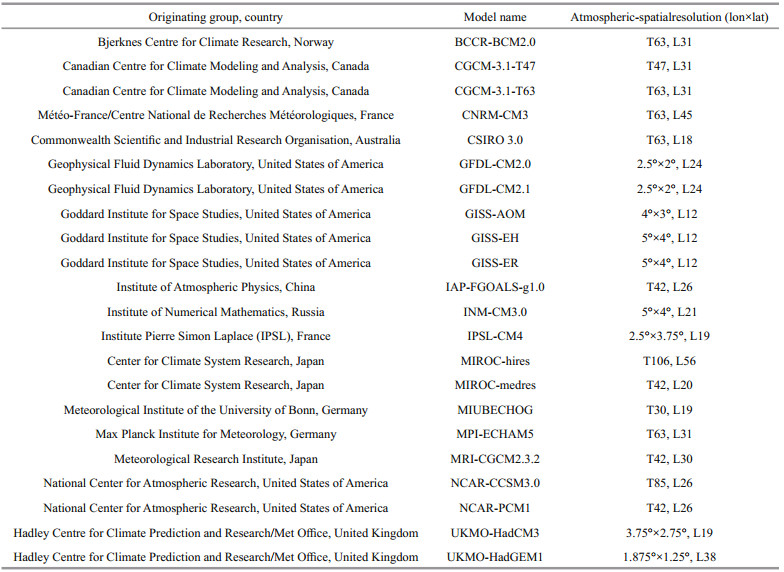
2.2 Multi-model outputsWe evaluate climate data from the coupled climate models of the CMIP3, which was used in the Intergovernmental Panel on Climate Change (IPCC) Fourth Assessment Report (AR4; Solomon et al., 2007) (Table 1).
|
Our analysis is based on outputs from three sets of simulations: 1) the pre-industrial control simulation (PI: CO2 concentration stabilizes at 360×10-6) representing the unforced natural variability of the climate system; 2) the 20th Century Climate in Coupled Models (20C3M) experiment, which incorporate anthropogenic and natural forcings from the observed atmospheric change in composition during the 20th century; 3) the Special Report on Emission Scenarios (SRES) A1B scenario, representing the most likely greenhouse gas emissions (CO2 concentration reaches 720×10-6 at the end of the 21st century and stabilizes afterward) of the global warming scenario in the 21st–22nd centuries.
In Section 3, we use the SLP output of 22 models from the 20C3M simulation to evaluate the simulation of the spatiotemporal features of the NPO in the 20th century. The models simulating both the geographic distribution and amplitude of NPO variability relatively well are chosen to further investigate the response of the NPO to global warming. Here, we compare model statistics from the SRES-A1B scenario with PI runs. In Section 4, we use the additional output of air temperature (Ta) to study atmospheric baroclinicity. Monthly-mean atmospheric fields are interpolated to a 2.5°×2.5° grid for both observational and multi-model data to facilitate comparisons between models of different spatial resolutions (Table 1).
To control temporal variables, we chose a 100-year period for both the PI control period (1901–2000) and SRES-A1B (2101–2200) scenario when CO2 levels stabilize (selecting the time that the models are running stably). Only one member (run1) of each model is used.
2.3 Methodology of constructing NPO pattern and its intensityThe primary method of constructing the principal component of SLP anomalies is empirical orthogonal function (EOF) analysis, which is defined by eigenvectors of the cross-covariance matrix between grid points (Lorenz, 1956), and aims to find uncorrelated linear combinations of different variables that explain maximum variance. Thus, a set of orthogonal spatial patterns and a set of associated uncorrelated time series or principal components are constructed when the spatiotemporal meteorological field is given (Hannachi et al., 2007).
The NPO index is defined as the second leading principal component (PC2) of the SLP anomalies in the region bounded by the area 10°–80°N and 120°E–90°W (Linkin and Nigam, 2008), which is also used to bound regression analyses and other general research on the NPO. For the NPO pattern, monthly anomalies are calculated by removing the climatology and linear trend in 100-year windows. Then, the anomalies are smoothed with a 3-month temporal filter to obtain the December–January– February (DJF) value of the NPO, which is generally persistent throughout the boreal winter months. Before the EOF analysis, the filtered fields are weighted by the square root of the cosine of latitude to account for the poleward decrease of grid area. The wintertime NPO pattern is derived by regression of the monthly DJF anomaly field onto the normalized PC2, which represents the typical NPO amplitude corresponding to one standard deviation of the principal component from the EOF analysis.
Based on the NPO pattern, we define the NPO intensity (NPOi) as a linear combination of centers of action,
 (1)
(1)where NPOai (northern lobe) and NPObi (southern lobe) denote intensities of the two centers of the NPO dipole, which are computed as a five-point mean (i.e., central maxima or minima plus four orthogonal values around the center point) of the central SLP anomaly value. A positive (negative) value of NPOi represents its positive (negative) phase, and only positive NPOi are used herein for a unified standard of NPO intensity between the SRES-A1B scenario and PI control simulations. Therefore, (-NPOai) and NPObi in Eq.1 are all positive values. While Wallace and Gutzler (1981) defined a West Pacific index using the 500-hPa geopotential height field corresponding to the NPO at SLP with a similar vertical structure (Linkin and Nigam, 2008), the steady locations used to measure centers of the patterns could not be used here to evaluate all the models on a consistent basis. This is because of the inherent bias unique to each model, which results in a different location of the center of action depending on the particular model. Therefore, we track every center location and extreme anomaly of the patterns to ensure NPOi comparability between different models.
Multi-model ensemble mean (MEM) statistics are calculated from the mean of the individual statistic analyzed. For example, the MEM pattern of the NPO is computed as the mean of individual patterns (adjusted to the positive phase) derived by regression of the SLP anomaly field in DJF onto the normalized NPO index from individual models.
3 RESULTHere, we analyze the NPO response to global warming from simulations of the future climate, with a focus on changes in intensity (see Section 2.3 for the definition of NPO intensity). First, models showing similar spatial patterns to observations are selected for assessment of the NPO response to global warming. Second, the internal NPO variability is tested to ensure the change is significant. Third, we inspect the changes of the NPO in those models that represent the observed spatial features well.
3.1 Multi-model selectionGiven the relatively modest role of observed greenhouse gas and aerosol forcing, simulations of the climate of the 20th century are a significant challenge for models, because of the difficulty in simulating natural variability as a result of the sensitivity to the initial and boundary conditions, as well as the uncertainty with the parameterization schemes and the degree of atmosphere-ocean coupling. Consequently, the outputs from models vary, for which the accurate portrayal of key features of the low-frequency NPO pattern is a first-order question. Therefore, we calculate the correlation coefficient R between the observed spatial pattern o and the spatial patterns of the 22 models m for the 20C3M simulation of the 1901–2000 period (the same period as the observations), where R is defined as:
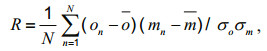 (2)
(2)where o and m are mean values and σo and σm are the standard deviations of o and m, respectively. Table 2 lists R and the normalized variance contributions (NVC) (i.e. the actual variance contribution of the models divided by the observations) of the principal component of each of the 22 IPCC AR4 models, showing the failure (R < 0.6) of the BCCR-BCM2.0 (R=0.09), GISS-EH (R=0.11), INM-CM3.0 (R=0.53) and UKMO-HadGEM1 (R=0.32) models to capture NPO patterns sufficiently. As the NVC is a standardized variance contribution, the NVC of the observed NPO pattern equals one; values much larger or smaller than one insufficiently capture the amplitude of NPO variability.
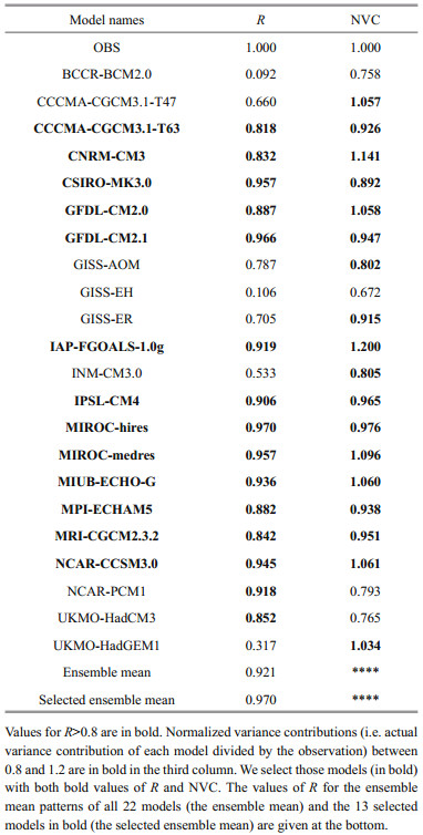
We find 13 models with R > 0.8 and NVC between 0.8 and 1.2 (CCCMA-CGCM3.1-T63, CNRM-CM3, CSIRO-MK3.0, GFDL-CM2.0, GFDL-CM2.1, IAPFGOALS-1.0g, IPSL-CM4, MIROC-hires, MIROCmedres, MIUB-ECHO-G, MPI-ECHAM5, MRICGCM2.3.2, NCAR-CCSM3.0) whose ensemble mean pattern (Fig. 1c) has a more similar spatial structure and greater correlation (Table 2) than that delivered by the ensemble of all 22 models (Fig. 1b), as compared with observations (Fig. 1a). For the temporal component, we correlate the observational time series of the EOF analysis with each model's time series to find (not shown) no correlation (R < 0.1, P > 0.1 for most models). Hence, while it is undeniable that temporal simulations of all IPCC-AR4 models are flawed, two models (CSIRO-Mk3.0 and UKMOHadGEM1) do give results above the 90% confidence level; correlations nonetheless remain < 0.15. Figure 1d shows normalized time series of the NPO from 22 models, along with the ensemble mean of 22 models (offset by +3), the ensemble mean of the 13 selected models (offset by -3), and observational indices, with correlations between the ensemble means and observations both < 0.1 (P > 0.1). Therefore, as the accuracy of the temporal simulation still needs improvement, our assessment of the NPO response to global warming mainly depends on those models with a reasonable spatial correspondence with observations.

|
| Figure 1 (a) Positive phase of the observed NPO (hPa) with dashed contours indicating negative values and solid contours positive values; as (b) but for the ensemble mean pattern of the 22 IPCC-AR4 models for the 20C3M experiment and (c) the ensemble mean pattern for the 13 selected models; (d) normalized principal components of multiple models for the 20C3M experiment and observations Black curve: NPO time series of observations; red curve: all 22 models (offset by +3); blue curve: 13 selected models (offset by -3) for the ensemble mean time series; gray thin lines: time series of all 22 IPCCAR4 models. |
To test the significance of the changes in the NPO variability as forced by global warming, the unforced internal variability in the PI simulation of each selected model is calculated. First, 500-year outputs of the PI run of each model (except MIROC-hires, which has only 100 years in the PI simulation) are used to create forty 100-year-length sliding windows (i.e., 001–100, 011–110, …, 401–500; where 001 is the initial year of the PI run). Then, 40 positive NPO patterns are derived from these 40 segments, which are considered independent of each other by assuming that the atmospheric states are uncorrelated. Indeed, no significant correlations of the time series between two consecutive segments are found upon further inspection. Finally, we compute the NPO intensity in each pattern, and use the standard deviation of the 40 intensities as the unforced internal variability of the NPO.
3.3 Response of the NPO to global warmingIn this section, we ascertain the NPO response to a warmer environment from the global warming simulation (SRES A1B). To facilitate comparisons between the SRES-A1B scenario and the PI control simulation of the NPO pattern, we present positive-phase NPO patterns of the 13 selected models in Fig. 2, with both PI and SRES-A1B simulations using the method described in Section 2.

|
| Figure 2 From top to bottom and left to right, are NPO dipole changes from most to least between the PI control and SRESA1B scenario for each of the 13 selected models A positive phase of NPO patterns for each model is used for comparison. Solid (dashed) contours stand for positive (negative) values of NPO dipole. |
Figure 2 displays patterns of NPO change by calculating the NPOi difference in each model between the SRES-A1B scenario and the PI control simulations, and then sequencing the models from the most change (largest percentage of the difference divided by NPOi in the PI run) to the least change (smallest percentage). After global warming, five models (CNRM-CM3, MIROC-medres, GFDLCM2.1, MRI-CGCM2.3.2, and MIUB-ECHO-G) show decreases in intensity of both the northern and southern lobes of the NPO dipole. Five other models (CCCMA-CGCM3.1-T63, CSIRO-MK3.0, MPIECHAM5, IAP-FGOALS-1.0g, and NCARCCSM3.0) reveal a reduced NPOa and enhanced NPOb. Two models (IPSL-CM4 and GFDL-CM2.0) present an increased NPOa and weakened NPOb. The MIROC-hires output is placed last because it shows little change in intensities of the NPO dipole. Therefore, as 10 of the 13 selected models show a weakened NPOa versus only 7 of the 13 selected models showing a weakened NPOb, the NPOa is considered more robust, which is consistent with an overall weakening of the NPO. We also find a westward shifting of the southern lobe (NPOb) in the results of three models (IPSL-CM4, GFDL-CM2.0, MIROC-medres, and MPI-ECHAM5), but an eastward shift for two models (GFDL-CM2.1 and CCCMA-CGCM3.1-T63). The remaining models indicate no zonal shift. The MEM patterns of the 13 selected models for the PI control and SRES-A1B scenario simulations are shown in the upper and middle panels of Fig. 3, along with the anomaly (A1B−PI) in the lower panel, which reveals a weakened NPO dipole.

|
| Figure 3 As in Fig. 2, but for MEM patterns (hPa) of the 13 selected models, along with the anomaly (lower panel, hPa) between the SRES-A1B scenario (middle panel) and PI control (upper panel) simulations |
Figure 4 depicts a summary of NPOi differences between the SRES-A1B scenario and the PI control from the patterns found in Fig. 2, and represents the change is NPO intensity resulting from global warming. The models are presented in the same order as Fig. 2 from left to right. Error bars show the internal variability of each model in the PI simulation via the aforementioned method. Because there are only onehundred years in the PI data of the MIROC-hires model, we could not determine its internal variability. As this model shows little change between the SRESA1B scenario and the PI control simulations, it is considered as an outlier here. The percentages displayed below the bars are computed by dividing the difference by the NPOi in the PI reference period. The NPOi differences of the MEM patterns (Fig. 3) is also calculated, with the error bars showing results significant at the 95% confidence level based on a two-tailed Student's t-test of the 13 models. The findings show that the NPO weakens in 12 of the 13 selected models, with 10 of the 12 models having significant results after global warming, and decreasing by more than ~10% in NPOi. The variance contributions of EOF-2 in 12 of the 13 models decreases for the SRES-A1B scenario with the exception of the MIROC-hires model, which increases by 2% from 0.195 to 0.199. That a clear and robust weakening of the NPO in response to global warming is evident motivates us to find the cause of this phenomenon.

|
| Figure 4 Bar graph showing NPOi differences between the SRES-A1B scenario and the PI control simulations of the 13 selected models, with the same sequence of models as Fig. 2 The error bars represent the internal variability (see Section 3.2) of each model, which is significant when the NPOi changes its internal variability. The percentages show an NPOi change (i.e., the difference divided by NPOi for the PI reference) in each model. The percentage difference of the MEM pattern located at the tips of the error bars indicate the results of Student's t-test of the 13 models listed for the 95% significance level. |
The momentum flux resulting from baroclinic eddies has been shown to influence large-scale midlatitude stirring associated with the North Atlantic Oscillation (Vallis et al., 2004), which has similarly been associated with the large-scale climate mode of the NPO (Di Lorenzo et al, 2013. Moreover, eddy formation is generally closely related to atmospheric baroclinicity (Nakamura, 1992). Such eddies are important in determining atmospheric circulation patterns via their interaction with the time-mean flow, interactions among themselves, and latitudinal transport of momentum and heat (e.g., Hoskins et al., 1983; Lau, 1988; Branstator, 1995).
To gauge the extent of NPO weakening, we consider all the models giving significant NPO weakening (CCCMA-CGCM3.1-T63, CNRM-CM3, CSIRO-MK3.0, GFDL-CM2.0, GFDL-CM2.1, IPSLCM4, MIROC-medres, MPI-ECHAM5, and MRICGCM2.3.2) according to Fig. 4 (i.e., an NPOi change exceeding its internal variability) except for the MIUB-ECHO-G model, which does not have atmospheric pressure-level data.
We transform center locations of the NPO dipole from the selected models into statistics to ascertain the zonal range of NPOa (NPOb) centers as 177.5°E (172.5°E) to 135°W (152.5°W) in both simulations of the PI control and the SRES-A1B scenario. We then use monthly Ta data to compute atmospheric baroclinicity over a zonal mean (170°E–130°W, i.e., containing the zonal range of both centers of the NPO) for the vertical (pressure levels: 1 000 hPa, 850 hPa, 500 hPa and 200 hPa) temperature difference between the SRESA1B scenario and PI reference from 10°N to 80°N (units ℃), which are shown in Fig. 5. We exclude the IPSL-CM4 model, whose output contains numerous missing values in the selected longitudinal band 40°N to 70°N at the 1 000- hPa and 850-hPa levels. The mean vertical shear of the zonal geostrophic wind (Nakamura, 1992) is given by:
 (3)
(3)where f0 is the Coriolis parameter at 45°N, g is the acceleration due to gravity, T is the air temperature, and U is the zonal wind. Here, we replace U and T with U', which is the zonal-wind difference between the SRES-A1B scenario and the PI control simulations, i.e., UA1B−UPI, and, similarly, T'=TA1B−TPI, respectively. The value of T in the Eq.3 is the mean air temperature in the selected area between certain vertical levels. Therefore, as g/f0T is a constant, the sign of ∂U/∂z depends on ∂T/∂y.
We see from all the models in Fig. 5 that T' > 0 and ∂T/∂y > 0 at mid-latitudes (i.e., the area between the two centers of the NPO dipole from about 30° to 70°N) below the 500-hPa level, which results in 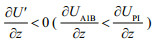

|
| Figure 5 Zonal mean (170°E–130°W) air temperature (Ta) difference between the SRES-A1B scenario and the PI control simulations from 10°N to 80°N (x-axis) at 1 000-hPa, 850-hPa, 500-hPa and 200-hPa levels (y-axis) (units: ℃) Center locations of the NPO dipole in the PI control (SRES-A1B scenario) are indicated by dashed (solid) straight lines. The MEM pattern is calculated by averaging the Ta differences of the eight models. |
By marking the center positions of the NPO dipole for the PI reference (SRES-A1B scenario) with dashed (solid) lines, we see that the NPO of most models shifts northward in the global-warming simulations. As mentioned above, the NPOa according to the GFDL-CM2.0 model is enhanced. From Fig. 5, NPOa centers in both the PI and SRES-A1B simulations of that model are located directly in the area of increased atmospheric baroclinicity (i.e., ∂U'/∂z > 0), which then shift southward. The incremental NPOb centers according to the CCCMACGCM3.1-T63, CSIRO-MK3.0 and MPI-ECHAM5 models are also situated in the enhanced baroclinicity area, but are also shifted northward. We hypothesize that the center of the northern lobe NPOa is located in an area of weaker baroclinity gradient than that for the southern lobe NPOb, thus leading to the northward movement of the NPO.
For further proof of the relationship between the weakening of the NPO and the decrease in atmospheric baroclinicity, Fig. 6 shows the linear correlation between the NPO intensity and baroclinicity. We also calculate the negative mean meridional gradient of surface air temperature difference (∂T'/∂y) from 25° to 75°N (the area containing the NPO dipole) representing the baroclinity change in each model, because other parameters (f0, g, and T) are constants in the Eq.3. Then, we compare ∂T'/∂y with the NPOi to find a robust correlation (R=0.8, P=0.01) between the two, demonstrating that the NPO weakening is mainly caused by the decrease in baroclinity.

|
| Figure 6 Scatter plot of negative mean meridional gradient of surface air temperature difference (x-axis) from 25° to 75°N versus changes in NPO intensity under global warming (y-axis) The blue line denotes the linear regression. The correlation between points is indicated in the upper part of the diagram. |
Global warming weakens the NPO dipole and shifts it further northward, which is mainly owing to the movement of NPOa, and is caused by a decrease in lower-tropospheric baroclinity in the mid-latitude North Pacific. Consequently, eddy activity is reduced, resulting in the transfer of less energy to the NPO.
5 CONCLUSIONThe second leading pattern of the SLP field in the boreal winter was explored with the help of 20CRv2 reanalysis data. A 100-year wintertime from 1901 to 2000 is extracted from monthly SLP data to reproduce the spatial structure of the NPO pattern via EOF and regression analyses, which enables direct visual inspection of the NPO for evaluation of model performance with respect to the observations.
The 20C3M simulations of the 22 IPCC AR4 models are used to evaluate the reconstruction of the spatial NPO pattern. By correlating each NPO pattern captured in the SLP anomaly field of each model, and comparing the variance contribution of each second mode of the EOF analysis with observations, we selected 13 models with superior MEM patterns to the 22 models together when compared with the observations. As there is little temporal correlation between the models and observations, we use the spatially generated NPO structure for assessment of model capability.
The NPO patterns of both the PI reference and SRES-A1B scenario simulations are used to evaluate the NPO response to higher average global temperatures based on the 13 selected models. To indicate the change in NPO pattern resulting from global warming, we define the NPO intensity NPOi for determining the strength of the spatial pattern delivered by each model. The different NPOi resulting from the SRES-A1B scenario and PI control simulations lead us to conclude that the NPO intensity both weakens and shifts northward as a result of global warming.
The cause of the weakened NPO is investigated through atmospheric baroclinicity, with eight models showing substantial reductions in baroclinicity during the SRES-A1B scenario, particularly in the lower troposphere over the mid-latitude North Pacific. A reduced baroclinicity in the lower troposphere transfers less energy and vorticity to the large and low-frequency scales of motion, thus leading to NPO weakening.
6 DATA AVAILABILITY STATEMENTThe 20th Century Reanalysis Version 2 data analyzed here are provided by NOAA/OAR/ESRL PSD, Boulder, Colorado, USA, via their website at http://www.esrl.noaa.gov/psd/.
Data from the IPCC AR4 models are available from the World Data Centre Climate (WDCC) at the German Climate Computing Centre (DKRZ), via their website at http://www.ipcc-data.org/sim/gcm_monthly/SRES_AR4/index.html.
7 ACKNOWLEDGEMENTThe authors acknowledge various modeling groups for making their simulations available for analysis, as well as the Program for Climate Model Diagnosis and Intercomparison (PCMDI) for collecting and archiving the CMIP3/IPCC AR4 model output.
Ashok K, Behera S K, Rao S A, Weng H Y, Yamagata T. 2007. El Niño Modoki and its possible teleconnection. J. Geophys. Res., 112(C11): C11007. DOI:10.1029/2006JC003798 |
Branstator G W. 1995. Organization of storm track anomalies by recurring low-frequency circulation anomalies. J.Atmos. Sci., 52(2): 207-226. DOI:10.1175/1520-0469(1995)052<0207:OOSTAB>2.0.CO;2 |
Cai M, Yang S, Van den Dool H M, Kousky V E. 2007. Dynamical implications of the orientation of atmospheric eddies:a local energetics perspective. Tellus A:Dynamic Meteorology and Oceanography, 59(1): 127-140. DOI:10.1111/j.1600-0870.2006.00213.x |
Chhak K C, Di Lorenzo E, Schneider N, Cummins P F. 2009. Forcing of low-frequency ocean variability in the Northeast Pacific. J. Climate, 22(5): 1 255-1 276. DOI:10.1175/2008JCLI2639.1 |
Compo G P, Whitaker J S, Sardeshmukh P D, Matsui N, Allan R J, Yin X, Gleason B E, Vose R S, Rutledge G, Bessemoulin P, Brönnimann S, Brunet M, Crouthamel R I, Grant A N, Groisman P Y, Jones P D, Kruk M C, Kruger A C, Marshall G J, Maugeri M, Mok H Y, Nordli Ø, Ross T F, Trigo R M, Wang X L, Woodruff S D, Worley S J. 2011. The twentieth century reanalysis project. Quart. J.Roy. Meteor. Soc., 137(654): 1-28. DOI:10.1002/qj.776 |
Di Lorenzo E, Cobb K M, Furtado J C, Schneider N, Anderson B T, Bracco A, Alexander M A, Vimont D J. 2010. Central Pacific El Niño and decadal climate change in the North Pacific Ocean. Nat. Geosci., 3(11): 762-765. DOI:10.1038/ngeo984 |
Di Lorenzo E, Combes V, Keister J E, Strub P T, Thomas A C, Franks P J S, Ohman M D, Furtado J C, Bracco A, Bograd S J, Peterson W T, Schwing F B, Chiba S, Taguchi B, Hormazabal S, Parada C. 2013. Synthesis of Pacific Ocean climate and ecosystem dynamics. Oceanography, 26(4): 68-81. DOI:10.5670/oceanog |
Di Lorenzo E, Schneider N, Cobb K M, Franks P J S, Chhak K, Miller A J, McWilliams J C, Bograd S J, Arango H, Curchitser E, Powell T M, Rivière P. 2008. North Pacific Gyre Oscillation links ocean climate and ecosystem change. Geophys. Res. Lett., 35(8): L08607. |
Hannachi A, Jolliffe I T, Stephenson D B. 2007. Empirical orthogonal functions and related techniques in atmospheric science:a review. Int. J. Climatol., 27(9): 1 119-1 152. DOI:10.1002/(ISSN)1097-0088 |
Hoskins B J, James I N, White G H. 1983. The shape, propagation and mean-flow interaction of large-scale weather systems. J. Atmos. Sci., 40(7): 1 595-1 612. DOI:10.1175/1520-0469(1983)040<1595:TSPAMF>2.0.CO;2 |
Lau N C. 1988. Variability of the observed midlatitude storm tracks in relation to low-frequency changes in the circulation pattern. J. Atmos. Sci., 45(19): 2 718-2 743. DOI:10.1175/1520-0469(1988)045<2718:VOTOMS>2.0.CO;2 |
Linkin M E, Nigam S. 2008. The North Pacific OscillationWest Pacific teleconnection pattern:mature-phase structure and winter impacts. J. Climate, 21(9): 1 979-1 997. DOI:10.1175/2007JCLI2048.1 |
Lorenz E N. 1956. Empirical orthogonal functions and statistical weather prediction. Department of Meteorology, Scientific Report No.1, MIT, Cambridge: p.1-49. |
Mak M, Cai M. 1989. Local barotropic instability. J. Atmos.Sci., 46(21): 3 289-3 311. DOI:10.1175/1520-0469(1989)046<3289:LBI>2.0.CO;2 |
Nakamura H. 1992. Midwinter suppression of baroclinic wave activity in the Pacific. J. Atmos. Sci., 49(17): 1 629-1 642. DOI:10.1175/1520-0469(1992)049<1629:MSOBWA>2.0.CO;2 |
Nigam S. 2003. Teleconnections. In: Holton J R, Pyle J A, Curry J A eds. Encyclopedia of Atmospheric Sciences. Academic Press, London. p. 2 243-2 269.
|
Rogers J C. 1990. Patterns of low-frequency monthly sea level pressure variability (1899-1986) and associated wave cyclone frequencies. J. Climate, 3(12): 1 364-1 379. DOI:10.1175/1520-0442(1990)003<1364:POLFMS>2.0.CO;2 |
Solomon S, Qin D, Manning M, Chen Z, Marquis M, Averyt K B, Tignor M, Miller H L. 2007. Climate Change 2007:the Physical Science Basis:Contribution of Working Group Ⅰ to the Fourth Assessment Report of the Intergovernmental Panel on Climate Change. Cambridge University Press, Cambridge UK.
|
Vallis G K, Gerber E P, Kushner P J, Cash B A. 2004. A mechanism and simple dynamical model of the North Atlantic Oscillation and annular modes. J. Atmos. Sci., 61(3): 264-280. DOI:10.1175/1520-0469(2004)061<0264:AMASDM>2.0.CO;2 |
Vimont D J, Wallace J M, Battisti D S. 2003. The seasonal footprinting mechanism in the Pacific:implications for ENSO. J. Climate, 16(16): 2 668-2 675. DOI:10.1175/1520-0442(2003)016<2668:TSFMIT>2.0.CO;2 |
Walker G T, Bliss E W. 1932. World weather V. Mem. Roy.Meteor. Soc., 44: 53-84. |
Wallace J M, Gutzler D S. 1981. Teleconnections in the geopotential height field during the Northern Hemisphere winter. Mon. Wea. Rev., 109(4): 784-812. DOI:10.1175/1520-0493(1981)109<0784:TITGHF>2.0.CO;2 |
Wettstein J J, Wallace J M. 2010. Observed patterns of monthto-month storm-track variability and their relationship to the background flow. J. Atmos. Sci., 67(5): 1 420-1 437. DOI:10.1175/2009JAS3194.1 |
Yu J Y, Kim S T. 2011. Relationships between extratropical sea level pressure variations and the central Pacific and eastern Pacific types of ENSO. J. Climate, 24(3): 708-720. DOI:10.1175/2010JCLI3688.1 |
| Ashok K, Behera S K, Rao S A, Weng H Y, Yamagata T, 2007. El Niño Modoki and its possible teleconnection. J. Geophys. Res., 112(C11): C11007. Doi: 10.1029/2006JC003798 |
| Branstator G W, 1995. Organization of storm track anomalies by recurring low-frequency circulation anomalies. J.Atmos. Sci., 52(2): 207–226. Doi: 10.1175/1520-0469(1995)052<0207:OOSTAB>2.0.CO;2 |
| Cai M, Yang S, Van den Dool H M, Kousky V E, 2007. Dynamical implications of the orientation of atmospheric eddies:a local energetics perspective. Tellus A:Dynamic Meteorology and Oceanography, 59(1): 127–140. Doi: 10.1111/j.1600-0870.2006.00213.x |
| Chhak K C, Di Lorenzo E, Schneider N, Cummins P F, 2009. Forcing of low-frequency ocean variability in the Northeast Pacific. J. Climate, 22(5): 1 255–1 276. Doi: 10.1175/2008JCLI2639.1 |
| Compo G P, Whitaker J S, Sardeshmukh P D, Matsui N, Allan R J, Yin X, Gleason B E, Vose R S, Rutledge G, Bessemoulin P, Brönnimann S, Brunet M, Crouthamel R I, Grant A N, Groisman P Y, Jones P D, Kruk M C, Kruger A C, Marshall G J, Maugeri M, Mok H Y, Nordli Ø, Ross T F, Trigo R M, Wang X L, Woodruff S D, Worley S J, 2011. The twentieth century reanalysis project. Quart. J.Roy. Meteor. Soc., 137(654): 1–28. Doi: 10.1002/qj.776 |
| Di Lorenzo E, Cobb K M, Furtado J C, Schneider N, Anderson B T, Bracco A, Alexander M A, Vimont D J, 2010. Central Pacific El Niño and decadal climate change in the North Pacific Ocean. Nat. Geosci., 3(11): 762–765. Doi: 10.1038/ngeo984 |
| Di Lorenzo E, Combes V, Keister J E, Strub P T, Thomas A C, Franks P J S, Ohman M D, Furtado J C, Bracco A, Bograd S J, Peterson W T, Schwing F B, Chiba S, Taguchi B, Hormazabal S, Parada C, 2013. Synthesis of Pacific Ocean climate and ecosystem dynamics. Oceanography, 26(4): 68–81. Doi: 10.5670/oceanog |
| Di Lorenzo E, Schneider N, Cobb K M, Franks P J S, Chhak K, Miller A J, McWilliams J C, Bograd S J, Arango H, Curchitser E, Powell T M, Rivière P, 2008. North Pacific Gyre Oscillation links ocean climate and ecosystem change. Geophys. Res. Lett., 35(8): L08607. |
| Hannachi A, Jolliffe I T, Stephenson D B, 2007. Empirical orthogonal functions and related techniques in atmospheric science:a review. Int. J. Climatol., 27(9): 1 119–1 152. Doi: 10.1002/(ISSN)1097-0088 |
| Hoskins B J, James I N, White G H, 1983. The shape, propagation and mean-flow interaction of large-scale weather systems. J. Atmos. Sci., 40(7): 1 595–1 612. Doi: 10.1175/1520-0469(1983)040<1595:TSPAMF>2.0.CO;2 |
| Lau N C, 1988. Variability of the observed midlatitude storm tracks in relation to low-frequency changes in the circulation pattern. J. Atmos. Sci., 45(19): 2 718–2 743. Doi: 10.1175/1520-0469(1988)045<2718:VOTOMS>2.0.CO;2 |
| Linkin M E, Nigam S, 2008. The North Pacific OscillationWest Pacific teleconnection pattern:mature-phase structure and winter impacts. J. Climate, 21(9): 1 979–1 997. Doi: 10.1175/2007JCLI2048.1 |
| Lorenz E N, 1956. Empirical orthogonal functions and statistical weather prediction. Department of Meteorology, Scientific Report No.1, MIT, Cambridge: p.1–49. |
| Mak M, Cai M, 1989. Local barotropic instability. J. Atmos.Sci., 46(21): 3 289–3 311. Doi: 10.1175/1520-0469(1989)046<3289:LBI>2.0.CO;2 |
| Nakamura H, 1992. Midwinter suppression of baroclinic wave activity in the Pacific. J. Atmos. Sci., 49(17): 1 629–1 642. Doi: 10.1175/1520-0469(1992)049<1629:MSOBWA>2.0.CO;2 |
| Nigam S. 2003. Teleconnections. In: Holton J R, Pyle J A, Curry J A eds. Encyclopedia of Atmospheric Sciences. Academic Press, London. p. 2 243-2 269. |
| Rogers J C, 1990. Patterns of low-frequency monthly sea level pressure variability (1899-1986) and associated wave cyclone frequencies. J. Climate, 3(12): 1 364–1 379. Doi: 10.1175/1520-0442(1990)003<1364:POLFMS>2.0.CO;2 |
| Solomon S, Qin D, Manning M, Chen Z, Marquis M, Averyt K B, Tignor M, Miller H L, 2007. Climate Change 2007:the Physical Science Basis:Contribution of Working Group Ⅰ to the Fourth Assessment Report of the Intergovernmental Panel on Climate Change. Cambridge University Press, Cambridge UK. |
| Vallis G K, Gerber E P, Kushner P J, Cash B A, 2004. A mechanism and simple dynamical model of the North Atlantic Oscillation and annular modes. J. Atmos. Sci., 61(3): 264–280. Doi: 10.1175/1520-0469(2004)061<0264:AMASDM>2.0.CO;2 |
| Vimont D J, Wallace J M, Battisti D S, 2003. The seasonal footprinting mechanism in the Pacific:implications for ENSO. J. Climate, 16(16): 2 668–2 675. Doi: 10.1175/1520-0442(2003)016<2668:TSFMIT>2.0.CO;2 |
| Walker G T, Bliss E W, 1932. World weather V. Mem. Roy.Meteor. Soc., 44: 53–84. |
| Wallace J M, Gutzler D S, 1981. Teleconnections in the geopotential height field during the Northern Hemisphere winter. Mon. Wea. Rev., 109(4): 784–812. Doi: 10.1175/1520-0493(1981)109<0784:TITGHF>2.0.CO;2 |
| Wettstein J J, Wallace J M, 2010. Observed patterns of monthto-month storm-track variability and their relationship to the background flow. J. Atmos. Sci., 67(5): 1 420–1 437. Doi: 10.1175/2009JAS3194.1 |
| Yu J Y, Kim S T, 2011. Relationships between extratropical sea level pressure variations and the central Pacific and eastern Pacific types of ENSO. J. Climate, 24(3): 708–720. Doi: 10.1175/2010JCLI3688.1 |