 2018, Vol. 36
Institute of Oceanology, Chinese Academy of Sciences
Article Information
- JIANG Lin(蒋琳), DONG Changming(董昌明), YIN Liping(尹丽萍)
- Cross-shelf transport induced by coastal trapped waves along the coast of East China Sea
- Chinese Journal of Oceanology and Limnology, 36(3): 630-640
- http://dx.doi.org/10.1007/s00343-018-7008-x
Article History
- Received Jan. 5, 2017
- accepted in principle Feb. 14, 2017
- accepted for publication Apr. 6, 2017


2 Oceanic Modeling and Observation Laboratory, Nanjing University of Information Science and Technology, Nanjing 210044, China;
3 Department of Atmospheric and Oceanic Sciences, University of California, Los Angeles, 90095, USA;
4 First Institute of Oceanography, State Oceanic Administration, Qingdao 266001, China;
5 Laboratory for Regional Oceanography and Numerical Modeling, Qingdao National Laboratory for Marine Science and Technology, Qingdao 266237, China
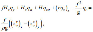
In shallow-sea dynamics, many dynamical phenomena occur in the coastal ocean over the continental shelf. Generally, pressure, wind, and precipitation induce sea level oscillations and current changes, which result in pollution transport and sediment resuspension, as well as mass transport over the shelf etc. In winter, Ekman transport and downwelling induced by the monsoons cause sediment to travel from the coast to the central continental shelf in the East China Sea (ECS) (Dong et al., 2011). In the Haizhou Bay nearshore in Jiangsu Province, the pollution diffuses offshore when the wind blows west-southwest (WSW), and accumulates onshore when the wind blows east (E) or eastsoutheast (ESE) (Xie et al., 2008). Simultaneously, onshore transport induced by nonlinear internal waves equals or exceeds offshore Ekman transport, so the internal waves play an important role on the material balance over the continental shelf (Zhang et al., 2015). These previous investigators have typically researched the mass transport on the continental shelf by numerical simulation or moored observations. There are still ambiguities in the theoretical mechanism of the transport on the continental shelf.
Cross-shelf transport can be caused by several physical processes, such as cross-shelf wind (Tilburg, 2003; Fewings et al., 2011) and nonlinear internal waves (Zhang et al., 2015). In China seas, the known inducing mechanism of cross-shelf transport includes the northerly monsoonal winds in the Yellow and East China Seas (Yuan and Hsueh, 2010) and nonlinear frontal waves (Liu et al., 2000).
In this paper, we start from the wind-driven coastal trapped waves (CTWs) mechanism to analyze the cross-shelf transport theoretically. CTWs are the hybrid waves with characteristics of both shelf waves and baroclinic Kelvin waves. They are formed along the coast due to the interactions of topography and stratification with the forcing (wind, tide and others) (Gill and Clark, 1974). CTWs can result in lowfrequency sea level fluctuations including generation in remote locations and propagation of the signals into the region (Hamon, 1962). The unidirectional propagation of CTWs along the coast can induce sea level changes of several centimeters (Gill and Schumann, 1974) and interface displacements of tens of meters (Colas et al., 2008). The vertical displacement enables elevation of nutrients into the euphotic zone to supply photosynthesis and profoundly impact primary production and the coastal ecological environment (Echevin et al., 2014). In China, the properties of CTWs in ECS and these waves' influence on the sea areas have been studied since the 1980s. Using hourly sea level records from tide stations and free CTWs theory, Chen and Su (1987) found free CTWs varied both seasonally and spatially in China seas. Hsueh and Pang (1989) studied the characteristics of wind-driven CTWs under the special double-shelf V-like bottom topography in the Yellow Sea, and pointed out lowfrequency sea-level signals propagating off both the east coast of China and the west coast of Korea. Using the ensemble empirical mode decomposition (EEMD) method, Yin et al. (2014) analyzed the observations from five mooring stations to confirm the existence of CTWs in the ECS with periods from 2 to 10 days. They found both alongshore wind stress and the curl of wind stress play an important role in the generation of CTWs. In winter 2008, Li et al. (2015) used observations including tidal records, alongshore winds, atmospheric pressure along the China coast, to show that winter storms can excite CTWs along the coast from Zhejiang to Guangdong southerly.
CTWs theory is comparatively well established, however, these researchers concentrate on the analysis of sea level observations and dynamics, and neglect their cross-shelf transport. Though the hindcast of onshore-offshore currents is underestimated based on the present CTWs theory (Brink, 1991), their role still has important theoretical significance. The wide continental shelf of the ECS is ecologically productive. CTWs are one of the primary factors that modify the near-shore currents over the shelf and shelf slope region, and CTWs play an important role in exchanging mass over the shelf (Huthnance, 1995). Weber and Drivdal (2012) found that barotropic CTWs induce the mean Lagrangian drift, which can be subdivided into a Stokes drift and a mean Eulerian drift, and CTWs make a profound influence on transporting biological material and displacing pollution. In this paper, we aim to analyze the crossshelf transport induced by wind-forced CTWs based on the previous studies. The rest of this paper is divided into the following sections: In Section 2, we briefly introduce the idealized wind-driven CTWs theory. Then we apply this theory to the ECS in Section 3. In an application, involving the study area, application with idealized wind stress and results. The discussion and summary are given in Section 4.
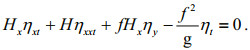
2 CTWS THEORYStarting with the barotropic, linearized and inviscid shallow-water equation, under the low-frequency and long-wave approximation, i.e. a wave frequency smaller than the inertial frequency (

 (1)
(1)subject to the boundary conditions:
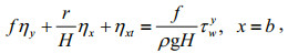 (2a)
(2a) (2b)
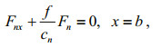
(2b)where x and y are the cross-shelf and alongshore coordinate respectively, t is the time, η(x, y, t) is the sea level change, g is the gravity acceleration, H is the water depth, f is the Coriolis parameter (taken as a constant), (τwx, τwy) is the wind stresses in x and y directions, respectively, r(x) is the bottom friction coefficient, r(x) can be simplified to be a constant in the calculation, and generally we let it be equal to 3×10⁻⁴ m/s when considering the weak damping. In Eq.2a, x=b is pretended to be the real coast, the depth of this cross-shelf location is equal to three times the Ekman layer e-folding scale δ (Clarke and Brink, 1985; Mitchum and Clarke, 1986), so this boundary condition indicates that there is no normal flow at the coast x=b, and Eq.2b states that the waves will vanish when x tends to infinite area, which means coastal trapping.
The properties of CTWs can be calculated by using a numerical model with realistic bottom topography. And η(x, y, t) can be divided into a cross-shelf distribution F(x) and an amplitude function ϕ(y, t) which vary along the coast and in time using the separation of variables method (Gill and Schumann, 1974)
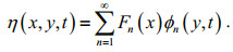 (3)
(3)Forced CTWs refer to a group of low frequency waves along the coastal area with the subscript n representing the wave mode.
The cross-shelf structure Fn(x) of the free waves can be solved using the following Sturm-Liouville eigenvalue equation (details see Appendix):
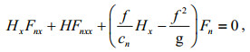 (4)
(4)subject to the boundary conditions:
 (5a)
(5a) (5b)
(5b)cn is the phase speed of the free wave to mode n, and its inverse is also the eigenvalue of this equation (Chapman, 1987).
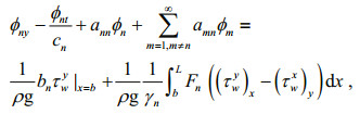
Amplitude function ϕ(y, t) satisfies an infinite set of coupling first-order wave equation according to the numerical method from Clarke and Van Gorder (1986)
 (6)
(6)where
 (7a)
(7a) (7b)
(7b) (7c)
(7c)where amn represent the frictional coupling coefficient to mode m in /m, and the reciprocal of ann provides the decay distance in the alongshore distance; bn is the wind-coupling coefficient. Since bottom friction effects are included, idealized winds must not be started abruptly, but phased in. The ramp-up or spinup time is equal to max 
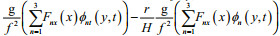
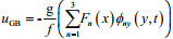
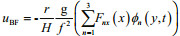
Two steps are required to solve the sea level change. First, we need to solve the cross-shelf structure Fn(x) and phase speed cn of the free waves, which is essential to calculate the free wave parameter amn, bn, and γn in Eq.7. Second, the amplitude function, ϕ(y, t), is solved numerically using these parameters. Once the sea level, η(x, y, t), is determined, the corresponding currents can be calculated following:
 (8a)
(8a) (8b)
(8b)According to Eq.8a, we can calculate the mean cross-shelf volume transport. We denote the mean variable by an over-bar, which is averaged over the wave period T. Mean cross-shelf seawater volume transport 
 (9)
(9) (10)
(10)where M denotes the seawater volume transport.
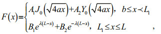
3 CTWS IN EAST CHINA SEA 3.1 Study areaFor the area around 29°N, where the Coriolis parameter is approximately equal to 7.0513×10⁻⁵/s. The Ryukyu Islands act as the wall in the ECS. We suppose the water depth H do not change with the straight coast y, and it is only the function of x. See Fig. 1, when the idealized water depth H are piecewise linear functions:
 (11)
(11)

|
| Figure 1 Idealized linearized topographic segment Here b=60 km, L1=430 km, L2=180 km, d=150 m, D=1 600 m. At the location x=b, the water depth is 21 m, which is equal to three times the Ekman layer e-folding scale δ. The location x=b is assumed to be the real coast. |
where α=d/L1, L=L1+L2. And in this figure, the crossshelf location x=b is pretended to be the real coast. Yin et al. (2014) set this water depth at the location x=b of each segment as 20 m, and here we set this water depth is 21 m. This cross section of the geometry is different from that in Chen and Su (1987), in which coast was set as x=0.
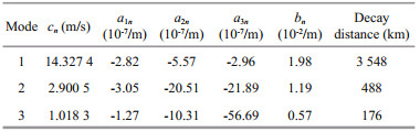
3.2 Application with idealized wind stressAffected by the monsoon, the nearshore of the ECS is driven by the north wind during winter. For simplification, we let τxw=0 and τyw=-0.07+ 0.03cos(l1y+w1t), where l1=3.64×10⁻⁶/m, w1=-3.64× 10⁻⁵/s. And we set Δy=1 000 m, Δx=1 000 m, and Δt=6 h in numerical calculation. CTWs refer to a group of low frequency waves along a coastal area, however, the selected modes are one of a subset of possible modes. Chapman (1987) pointed out that the higher the modes were more sensitive to the parameters, such as topography and bottom friction etc. This meant more modes could not improve the accuracy of the calculation. For study of the ECS, both Hsueh and Pang (1989) and Yin et al. (2014) believed the first three modes were sufficient to represent the dynamics. Yin et al. (2014) noted that combination of the first three modes replicated 90.3% of what was covered by the first six modes. Consequently, our analysis considers the first three modes. The first three modes of free wave F(x) are shown in Fig. 2. The lowest mode is called the KW mode, whose amplitude generally decays exponentially cross the shelf (blue in Fig. 2), and its phase speed is the largest, being about 14.3 m/s, which is close to 14.2 m/s in the table of Chen and Su (1987). The second and third modes are known as the shelf waves modes (SW1 and SW2) (green and red in Fig. 2, respectively), whose phase speed are 2.9 m/s and 1.02 m/s respectively, which are much smaller than the KW mode, and their amplitudes are different from the KW mode and generally decay in the wave form. In Fig. 2, x=430 km is the continental shelf break, and these three modes are almost zero beyond it. The change of the waves is mainly confined to the continental shelf. From Table 1, we find the decay distance of SW1 (488 km) and SW2 (176 km) is much shorter than KW (3 548 km). According to max= (-1/cnann), we know the spin-up time is about 69 hour.

|
| Figure 2 The cross-shelf structure for first three modes of the free waves, i.e. Fn(x) and the amplitudes are normalized with values set to 1 at the coast KW means Kelvin wave mode, SW1 and SW2 mean the first and second Shelf wave respectively. |
|
a) Flow decomposition
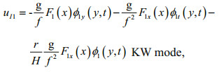
For the cross-shelf velocity, we divide it into two components according to Eq.8a. The first component is the interior flow, i.e. 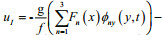


The spatial distribution of the cross-shelf transport attributable to the different terms in Eq.9 is shown in Fig. 3. The positive values represent offshore transport while the negative values represent onshore transport. The order of the SOW term (10-3) is much smaller than that of the others (10-1–1), so it can be ignored. The GB term (Fig. 3a) continually contributes to the offshore transport, which peaks at the coast, decreasing in magnitude and finally switching to onshore transport near about 300 km offshore. The effect of the BF term (Fig. 3c) is concentrated within 60–240 km offshore, and the offshore transport decreases with the cross-shelf distance. Figure 3d shows the spatial distribution of the total cross-shelf transport involving 4 terms, which increases along the crossshelf direction. Overall, we find the influence of the BF term is confined to 60–240 km offshore, while the contribution of the GB term covers over the whole continental shelf (Fig. 3).

|
| Figure 3 The spatial distribution of the cross-shelf transport attributable to GB term (a), SOW term (b), BF term (c) and all terms (d) The positive values represent offshore transport while the negative values represent onshore transport. |
The cross-shelf transport attributable to the different modes for each term in Eq.10 is shown in Fig. 4. For the GB term (Fig. 4a), KW and SW1 are dominant. The offshore transport attributable to the GB term peaks about 0.30 Sv at 81 km, then decays and turns into onshore transport at 376 km. For the GB term, the offshore transport attributable to the KW mode peaks about 0.33 Sv at 165 km, and the onshore transport attributable to the SW1 mode peaks about -0.27 Sv at 269 km. Though the contribution of the SOW term (Fig. 4b) can be overlooked, it is also the result of a combination of the three modes. The offshore transport attributable to the BF term (Fig. 4c) focuses on the nearshore between 60 and 240 km, and peaks about 0.26 Sv at the coast. In the BF term, the offshore transport induced by the KW mode peaks about 0.07 Sv at the coast and slowly decays to 0.02 Sv. The cross-shelf transport induced by the SW1 and SW2 modes both peak at the coast, about 0.12 Sv and 0.07 Sv, respectively. Figure 4d shows the cross-shelf transport attributable to four terms and the total cross-shelf transport attributable to all terms. Because of idealized wind stress, the cross-shelf transport induced by the EK term is constant at about 0.60 Sv along cross-shelf distance. The total crossshelf transport (red dotted line) is controlled by the GB, BF and EK term between 60 and 240 km, while the GB and EK terms are dominant from 240 km to the continental shelf margin. The total cross-shelf transport increases along the cross-shelf direction, and peaks about -0.73 Sv at the continental shelf margin.

|
| Figure 4 The cross-shelf transport attributable to different modes in GB term (a), SOW term (b) and BF term (c), and the cross-shelf transport attributable to different terms (d) The positive values represent offshore transport while the negative values represent onshore transport. |
b) Mode decomposition
Dividing uI into three modes, we call

an well as 
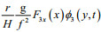
The spatial distribution of the cross-shelf transport attributable to the different modes in Eq.9 is shown in Fig. 5. The orders of these three modes are similar. For the spatial distribution, the offshore transport induced by the KW mode (Fig. 5a) increases along the crossshelf distance nearshore, and peaks between 100 and 200 km offshore, then slowly decreases in magnitude before finally switching to onshore transport near the continental shelf margin. Likewise, the alongshore transport attributable to the KW mode is generally constant in alongshore distance, and this satisfies that the bottom friction has little effect on the KW mode according to the decay distance of KW (3 548 km). The cross-shelf transport induced by the SW1 mode (Fig. 5b) fluctuates along the cross-shelf distance, and the offshore transport decreases along the cross-shelf distance between 60 and 150 km and then changes to the onshore transport. The cross-shelf transport induced by the SW2 mode (Fig. 5c) is similar to that induced by the SW1 mode, which has the trend of fluctuation along the cross-shelf distance, and the change is confined to the alongshore distance 0–180 km, consistent with the frictional decay distance of the SW2 in Table 1.

|
| Figure 5 The spatial distribution of the cross-shelf transport attributable to KW mode (a), SW1 mode (b), SW2 mode (c) and all terms (d) The positive values represent offshore transport while the negative values represent onshore transport. |
The cross-shelf transport attributable to the different terms for each mode in Eq.10 is shown in Fig. 6. The effect of the SOW term in each mode is weak, so it can be ignored. This is consistent with Fig. 3. For the KW mode, the GB term dominates and first increases peaking with an offshore transport of 0.38 Sv at 158 km offshore, then decreases with distance from the coast starting at 387 km (Fig. 6a). In the SW1 mode, the GB and BF terms dominate between 60 and 240 km. After 240 km, solely the GB term controls the flow (Fig. 6b). The cross-shelf transport induced by the SW1 mode changes from offshore to onshore at 136 km and peaks in onshore transport at -0.29 Sv at 289 km. For the SW2 mode, the GB and BF terms dominate the cross-shelf transport, which ranges widely from -0.05 Sv to 0.10 Sv (Fig. 6c). The cross-shelf transport caused both by three modes and the total including all terms are shown in Fig. 6d. Compared with the other two modes, SW2 mode's contribution to the total crossshelf transport is limited.

|
| Figure 6 The cross-shelf transport attributable to different terms in KW mode (a), SW1 mode (b) and SW2 mode (c), and the cross-shelf transport caused by different modes (d) The positive values represent offshore transport while the negative values represent onshore transport. |
c) Sensitivity to bottom friction
Wang et al. (1988) pointed out that the decay time of CTWs was about 3 days with bottom friction along the China coast. In this part, we will discuss the effects of different bottom friction coefficients r on the crossshelf transport. We take 4 different values of r (0, 3×10⁻⁴, 6×10⁻⁴ and 9×10⁻⁴ m/s) with the outputs shown in Fig. 7. In contrast to the other three conditions, the corresponding cross-shelf transport of the condition r=0 shows declining wave-like fluctuation with two peaks: one at the coast and the other at 180 km. The cross-shelf transport declines with distance with the slope becoming more uniform as r increases. The cross-shelf transport is generally affected by the bottom topography and the wind stress and energy originates primarily from wind stress, if bottom friction is neglected. However, with bottom friction, the transport is significantly attenuated.

|
| Figure 7 The sensitivity test for the mean cross-shelf transport of different bottom friction coefficients |
Theoretically, there is no normal flow at the coastal wall (x=b), i.e. the velocities and transport should equal zero, however, this is not true in the results. The number of selected modes is instrumental in determining the normal flow at the wall. As shown in Fig. 8, compared with the sum of the first three modes, the results of the sum of the first six modes is closer to 0 at the coast. But the results are similar to when a cross-shelf distance of 90 km is reached and diverge after 430 km. In addition, the results are more sensitive to the parameters due to selecting the higher order of the modes. This calculated error is therefore inevitable. According to the boundary condition of Eq.2a at x=b, the left equation actually include all the modes while the right part just relate to the wind stress, so considering only the first three modes may cause the left value to be slightly smaller than the right value. Further, as r increases this difference between the two sides becomes smaller until it reaches 0. This is the reason why the transport at x=b is closer to 0 with the increase of r in Fig. 7.

|
| Figure 8 Comparing the effect of the number of selected modes on the cross-shelf transport at the real coast |
In this paper, we investigate the role of CTWs in cross-shelf transport theoretically, and discuss the properties of the cross-shelf transport induced by wind-driven CTWs in the ECS in detail. According to the special topography profile in the ECS, we solve the cross-shelf structure of free waves, phase speed and free waves parameters of CTWs. Based on free waves, we apply the idealized wind stress to hindcast the cross-shelf current produced by wind-driven CTWs, and estimate the cross-shelf transport quantitatively. Assuming a barotropic ocean, this paper approaches the problem from two aspects. One is flow decomposition; the current is composed of 2 kinds of flow, i.e., interior flow and Ekman flow. The interior flow can be further divided into three terms: GB, SOW and BF terms. In other words, there are 4 terms. The other is mode decomposition; the current of interior component can be further divided into 3 modes: KW, SW1and SW2 modes.
(1) For the 4 terms, the SOW term can be ignored as it is small on the order of 10-3 while others are on the order of 10-1–1. The cross-shelf transport is controlled by the GB, BF and EK term from the coast to the central continental shelf, while the GB and EK term dominate from the central continental shelf to the continental shelf margin.
(2) For the 3 modes, because the decay distance of SW1 and SW2 is shorter than that of KW, the transport distributions produced by these two modes have some limitations in alongshore distance. And the effect of SW2 is weak compared with the other two modes, while the cross-shelf transport is mainly controlled by the KW and SW1 modes.
(3) The results show that the total cross-shelf transport travels onshore under the idealized wind stress on the order of 10-1, and it increases along the cross-shelf direction with the increased gradient decreasing, and peaks about -0.73 Sv at the continental shelf margin.
(4) In the discussion of sensitivity to bottom friction r, with the increase of r, the fluctuating trend of corresponding cross-shelf transport is getting weaker until it becomes approximately a smooth diagonal. And we think the outputs error at the coast, which is not equal to 0, mainly results from the number of selected modes. By comparing two conditions, namely the first three modes and the first six modes, we find that the results of the sum of the first six modes is closer to 0 at the coast than that of the first three modes. But the results are similar in cross-shelf distance 90–430 km.
This paper brought some significant insights on the role of CTWs and their contribution to the cross-shelf transport in the ECS. However, there is still a big gap in the understanding of this new mechanism, thus leaving rooms for more extensive research to be done on the subject, such as making the Coriolis parameter variable instead of constant and bottom friction is quadratic instead of being linear. Therefore, future research work will focus on these two aspects, as well as apply numerical simulations to investigate the cross-shelf transport induced by wind-driven CTWs, while also considering stratification condition.
5 ACKNOWLEDGEMENTThe authors would like to thank Prof. Liang, Prof. Weber, Prof. Wang and Kenny for their kindly help in this work.
APPENDIXFree CTWs structure Fn(x)
Dropping the forcing term of Eq.1, we obtain
 (A1)
(A1)We suppose η(x, y, t) can be divided into a cross-shelf distribution F(x) and an alongshore amplitude function ϕ(y, t), i.e. η(x, y, t)=F(x)ϕ(y, t), and we obtain a familiar eigenvalue problem in terms of F(x) (c is the phase speed of free CTWs and c=w/l):

Then see Fig. 1, substitute Eq.11 into Eq.4, we can obtain
 (A2)
(A2)where 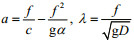
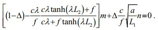 (A3)
(A3)
Then Eq.A3 can be solved numerically. There are infinite number of discrete values of cn (n=1, 2, …), which have the corresponding free wave modes, i.e. Fn(x).
Brink K H. 1991. Coastal-trapped waves and wind-driven currents over the continental shelf. Annual Review of Fluid Mechanics, 23(1): 389-412. DOI:10.1146/annurev.fl.23.010191.002133 |
Chapman D C. 1987. Application of wind-forced, long, coastal-trapped wave theory along the California coast. Journal of Geophysical Research:Oceans, 92(C2): 1 798-1 816. DOI:10.1029/JC092iC02p01798 |
Chen D K, Su J L. 1987. Continental shelf waves along the coasts of China. Acta Oceanologica Sinica, 6(3): 317-334. |
Clarke A J, Brink K H. 1985. The response of stratified, frictional flow of shelf and slope waters to fluctuating large-scale, low-frequency wind forcing. Journal of Physical Oceanography, 15(4): 439-453. DOI:10.1175/1520-0485(1985)015<0439:TROSFF>2.0.CO;2 |
Clarke A J, Van Gorder S. 1986. A method for estimating winddriven frictional, time-dependent, stratified shelf and slope water flow. Journal of Physical Oceanography, 16(6): 1 013-1 028. DOI:10.1175/1520-0485(1986)016<1013:AMFEWD>2.0.CO;2 |
Colas F, Capet X, Mcwilliams J C, et al. 2008. 1997-1998 El Niño off Peru:a numerical study. Progress in Oceanography, 79(2-4): 138-155. DOI:10.1016/j.pocean.2008.10.015 |
Dong L X, Guan W B, Chen Q, et al. 2011. Sediment transport in the Yellow Sea and East China Sea. Estuarine, Coastal and Shelf Science, 93(3): 248-258. DOI:10.1016/j.ecss.2011.04.003 |
Echevin V, Albert A, Lévy M, et al. 2014. Intraseasonal variability of nearshore productivity in the Northern Humboldt Current System:the role of coastal trapped waves. Continental Shelf Research, 73: 14-30. DOI:10.1016/j.csr.2013.11.015 |
Fewings M, Lentz S J, Fredericks J. 2011. Observations of cross-shelf flow driven by cross-shelf winds on the inner continental shelf. Journal of Physical Oceanography, 38(11): 2 358-2 378. |
Gill A E, Clarke A J. 1974. Wind-induced upwelling, coastal currents and sea-level changes. Deep Sea Research and Oceanographic Abstracts, 21(5): 325-345. DOI:10.1016/0011-7471(74)90038-2 |
Gill A E, Schumann E H. 1974. The generation of long shelf waves by the wind. Journal of Physical Oceanography, 4(1): 83-90. DOI:10.1175/1520-0485(1974)004<0083:TGOLSW>2.0.CO;2 |
Hamon B V. 1962. The spectrums of mean sea level at Sydney, Coff's Harbour, and Lord Howe Island. Journal of Geophysical Research, 67(13): 5 147-5 155. DOI:10.1029/JZ067i013p05147 |
Hsueh Y, Pang I C. 1989. Coastally trapped long waves in the Yellow Sea. Journal of Physical Oceanography, 19(5): 612-625. DOI:10.1175/1520-0485(1989)019<0612:CTLWIT>2.0.CO;2 |
Huthnance J M. 1995. Circulation, exchange and water masses at the ocean margin:the role of physical processes at the shelf edge. Progress in Oceanography, 35(4): 353-431. DOI:10.1016/0079-6611(95)80003-C |
Li J Y, Zheng Q A, Hu J Y, et al. 2015. Wavelet analysis of coastal-trapped waves along the China coast generated by winter storms in 2008. Acta Oceanologica Sinica, 34(11): 22-31. DOI:10.1007/s13131-015-0701-0 |
Liu K K, Tang T Y, Gong G C, et al. 2000. Cross-shelf and along-shelf nutrient fluxes derived from flow fields and chemical hydrography observed in the southern East China Sea off northern Taiwan. Continental Shelf Research, 20(4-5): 493-523. DOI:10.1016/S0278-4343(99)00083-7 |
Mitchum G T, Clarke A J. 1986. The frictional Nearshore response to forcing by synoptic scale winds. Journal of Physical Oceanography, 16(5): 934-946. DOI:10.1175/1520-0485(1986)016<0934:TFNRTF>2.0.CO;2 |
Tilburg C E. 2003. Across-shelf transport on a continental shelf:do across-shelf winds matter?. Journal of Physical Oceanography, 33(12): 2 675-2 688. DOI:10.1175/1520-0485(2003)033<2675:ATOACS>2.0.CO;2 |
Wang J, Yuan L Y, Pan Z D. 1988. Numerical studies and analysis about continental shelf waves. Acta Oceanologica Sinica, 10(6): 666-677. |
Weber J E H, Drivdal M. 2012. Radiation stress and mean drift in continental shelf waves. Continental Shelf Research, 35: 108-116. DOI:10.1016/j.csr.2012.01.001 |
Xie F, Pang Y, Zhuang W, et al. 2008. Study on regularity of matter transportation in the Nearshore Area of the Haizhou Bay. Advances in Marine Science, 26(3): 347-353. |
Yin L P, Qiao F L, Zheng Q A. 2014. Coastal-trapped waves in the East China Sea observed by a mooring array in winter 2006. Journal of Physical Oceanography, 44(2): 576-590. DOI:10.1175/JPO-D-13-07.1 |
Yuan D L, Hsueh Y. 2010. Dynamics of the cross-shelf circulation in the Yellow and East China Seas in winter. Deep Sea Research Part Ⅱ:Topical Studies in Oceanography, 57(19-20): 1 745-1 761. DOI:10.1016/j.dsr2.2010.04.002 |
Zhang S, Alford M H, Mickett J B. 2015. Characteristics, generation and mass transport of nonlinear internal waves on the Washington continental shelf. Journal of Geophysical Research:Oceans, 120(2): 741-758. DOI:10.1002/2014JC010393 |
| Brink K H, 1991. Coastal-trapped waves and wind-driven currents over the continental shelf. Annual Review of Fluid Mechanics, 23(1): 389–412. Doi: 10.1146/annurev.fl.23.010191.002133 |
| Chapman D C, 1987. Application of wind-forced, long, coastal-trapped wave theory along the California coast. Journal of Geophysical Research:Oceans, 92(C2): 1 798–1 816. Doi: 10.1029/JC092iC02p01798 |
| Chen D K, Su J L, 1987. Continental shelf waves along the coasts of China. Acta Oceanologica Sinica, 6(3): 317–334. |
| Clarke A J, Brink K H, 1985. The response of stratified, frictional flow of shelf and slope waters to fluctuating large-scale, low-frequency wind forcing. Journal of Physical Oceanography, 15(4): 439–453. Doi: 10.1175/1520-0485(1985)015<0439:TROSFF>2.0.CO;2 |
| Clarke A J, Van Gorder S, 1986. A method for estimating winddriven frictional, time-dependent, stratified shelf and slope water flow. Journal of Physical Oceanography, 16(6): 1 013–1 028. Doi: 10.1175/1520-0485(1986)016<1013:AMFEWD>2.0.CO;2 |
| Colas F, Capet X, Mcwilliams J C, et al, 2008. 1997-1998 El Niño off Peru:a numerical study. Progress in Oceanography, 79(2-4): 138–155. Doi: 10.1016/j.pocean.2008.10.015 |
| Dong L X, Guan W B, Chen Q, et al, 2011. Sediment transport in the Yellow Sea and East China Sea. Estuarine, Coastal and Shelf Science, 93(3): 248–258. Doi: 10.1016/j.ecss.2011.04.003 |
| Echevin V, Albert A, Lévy M, et al, 2014. Intraseasonal variability of nearshore productivity in the Northern Humboldt Current System:the role of coastal trapped waves. Continental Shelf Research, 73: 14–30. Doi: 10.1016/j.csr.2013.11.015 |
| Fewings M, Lentz S J, Fredericks J, 2011. Observations of cross-shelf flow driven by cross-shelf winds on the inner continental shelf. Journal of Physical Oceanography, 38(11): 2 358–2 378. |
| Gill A E, Clarke A J, 1974. Wind-induced upwelling, coastal currents and sea-level changes. Deep Sea Research and Oceanographic Abstracts, 21(5): 325–345. Doi: 10.1016/0011-7471(74)90038-2 |
| Gill A E, Schumann E H, 1974. The generation of long shelf waves by the wind. Journal of Physical Oceanography, 4(1): 83–90. Doi: 10.1175/1520-0485(1974)004<0083:TGOLSW>2.0.CO;2 |
| Hamon B V, 1962. The spectrums of mean sea level at Sydney, Coff's Harbour, and Lord Howe Island. Journal of Geophysical Research, 67(13): 5 147–5 155. Doi: 10.1029/JZ067i013p05147 |
| Hsueh Y, Pang I C, 1989. Coastally trapped long waves in the Yellow Sea. Journal of Physical Oceanography, 19(5): 612–625. Doi: 10.1175/1520-0485(1989)019<0612:CTLWIT>2.0.CO;2 |
| Huthnance J M, 1995. Circulation, exchange and water masses at the ocean margin:the role of physical processes at the shelf edge. Progress in Oceanography, 35(4): 353–431. Doi: 10.1016/0079-6611(95)80003-C |
| Li J Y, Zheng Q A, Hu J Y, et al, 2015. Wavelet analysis of coastal-trapped waves along the China coast generated by winter storms in 2008. Acta Oceanologica Sinica, 34(11): 22–31. Doi: 10.1007/s13131-015-0701-0 |
| Liu K K, Tang T Y, Gong G C, et al, 2000. Cross-shelf and along-shelf nutrient fluxes derived from flow fields and chemical hydrography observed in the southern East China Sea off northern Taiwan. Continental Shelf Research, 20(4-5): 493–523. Doi: 10.1016/S0278-4343(99)00083-7 |
| Mitchum G T, Clarke A J, 1986. The frictional Nearshore response to forcing by synoptic scale winds. Journal of Physical Oceanography, 16(5): 934–946. Doi: 10.1175/1520-0485(1986)016<0934:TFNRTF>2.0.CO;2 |
| Tilburg C E, 2003. Across-shelf transport on a continental shelf:do across-shelf winds matter?. Journal of Physical Oceanography, 33(12): 2 675–2 688. Doi: 10.1175/1520-0485(2003)033<2675:ATOACS>2.0.CO;2 |
| Wang J, Yuan L Y, Pan Z D, 1988. Numerical studies and analysis about continental shelf waves. Acta Oceanologica Sinica, 10(6): 666–677. |
| Weber J E H, Drivdal M, 2012. Radiation stress and mean drift in continental shelf waves. Continental Shelf Research, 35: 108–116. Doi: 10.1016/j.csr.2012.01.001 |
| Xie F, Pang Y, Zhuang W, et al, 2008. Study on regularity of matter transportation in the Nearshore Area of the Haizhou Bay. Advances in Marine Science, 26(3): 347–353. |
| Yin L P, Qiao F L, Zheng Q A, 2014. Coastal-trapped waves in the East China Sea observed by a mooring array in winter 2006. Journal of Physical Oceanography, 44(2): 576–590. Doi: 10.1175/JPO-D-13-07.1 |
| Yuan D L, Hsueh Y, 2010. Dynamics of the cross-shelf circulation in the Yellow and East China Seas in winter. Deep Sea Research Part Ⅱ:Topical Studies in Oceanography, 57(19-20): 1 745–1 761. Doi: 10.1016/j.dsr2.2010.04.002 |
| Zhang S, Alford M H, Mickett J B, 2015. Characteristics, generation and mass transport of nonlinear internal waves on the Washington continental shelf. Journal of Geophysical Research:Oceans, 120(2): 741–758. Doi: 10.1002/2014JC010393 |