 2018, Vol. 36
Institute of Oceanology, Chinese Academy of Sciences
Article Information
- LU Zongze(陆宗泽), FAN Wei(樊伟), LI Shuang(李爽), GE Jianzhong(葛建忠)
- Large-eddy simulation of the influence of a wavy lower boundary on the turbulence kinetic energy budget redistribution
- Chinese Journal of Oceanology and Limnology, 36(4): 1178-1188
- http://dx.doi.org/10.1007/s00343-018-7015-y
Article History
- Received Apr. 7, 2017
- accepted in principle Jun. 12, 2017
- accepted for publication Jul. 13, 2017


2 State Key Laboratory of Estuarine and Coastal Research, East China Normal University, Shanghai 200062, China
Coastal water is always well mixed compared with deep ocean water. While relatively well-mixed coastal water promotes the generation of coastal flow (Li et al., 2005), coastal mixing does not remove the vertical current profile, implying that turbulence mixing still requires appropriate modeling. Models based on Reynolds-averaged Navier-Stokes (RANS) equations were used to describe coastal vertical mixing in early studies, which either parameterized the ocean turbulence as a bulk quantity (Large et al., 1994; Large and Gent, 1999; McWilliams and Sullivan, 2000; Smyth et al., 2002; Wijesekera et al., 2003) or used specific parameterizations of terms of the differential equations (Mellor and Yamada, 1982; Wilcox, 1988; Umlauf and Burchard, 2003). While RANS models assume that the turbulence can be characterized by the background low-frequency flow, or by the degree of convective instability, this assumption results in excessive noise and does not capture the nature of the turbulence. In response, the coastal turbulence study of Zeng et al. (2008) proposed a turbulence-resolving model to correct the uncertainty of RANS models.
Large-eddy simulations (LES) have produced successful numerical solutions of coastal turbulence (Li et al., 2013, 2016; Walker et al., 2016). For example, for small-scale unstable flow above sand grains, Chang and Scotti (2004) compared a RANS model with an LES model to show similar results for only the vertical variation of the streamwise velocity component, with obvious differences in the vertical velocity component, turbulence kinetic energy (TKE) budget, and other higher-order quantities. The study concluded that the RANS model is not suitable for simulating suspended sediment transport, while the LES model gives more accurate results in agreement with the findings of experiments in a laboratory setting.
Large-eddy simulation is commonly used to study the flow over wavy lower boundaries (Broglia et al., 2003; Grigoriadis et al., 2012, 2013; Harris and Grilli, 2012; Soldati and Marchioli, 2012) such as over sand ripples and sandbanks, which are very common in coastal waters and have a strong influence on sediment transport and wave energy dissipation.
Jackson and Hunt (1975) investigated the turbulent flow of air over hilly terrain in the laboratory, and showed that the flow acceleration reached a maximum above the hilltop, with the velocity over the top of the hill equal to the velocity at the upwind side of the hill at the same height. Henn and Sykes (1999) performed an LES of the flow over a rippled surface, and concluded that large spanwise fluctuations occur on the upslope boundary, and a detached shear layer exists in the lee of the crest, resulting in strong turbulence over the trough. Calhoun and Street (2001) also studied turbulent flow over a wavy surface, and showed that turbulence parameters above the valleys, such as turbulence intensity, turbulence transport and dissipation, and TKE, are larger than those above the hill tops. However, the mechanism behind the observed phenomena is still unclear.
Therefore, we use an LES model to explore the influence of a wavy seabed on the spatial distribution of the velocity and redistribution of the TKE budget, with Section 2 describing the LES model, and introducing the initial and boundary conditions, as well as important parameter settings. Section 3 presents an analysis of the simulation results, with a discussion and conclusions presented in Sections 4 and 5, respectively.
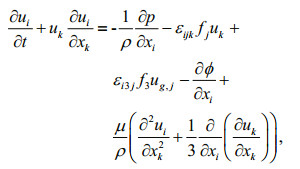
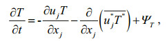
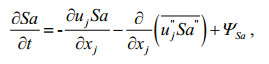
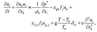
2 THEORY 2.1 Model descriptionThe LES model used here is the PArallelized Large-Eddy Simulation Model (PALM) for Atmospheric and Oceanic Flows, which was developed by the Institute of Meteorology and Climatology of Leibniz University, Germany. In general, LES is based on the spatial average of the turbulent fluctuations, which are divided into large-scale and small-scale eddies using a specified filter function. The large-scale eddies are then directly simulated, while the small-scale eddies are parameterized (Maronga et al., 2015). The basic governing equations for the LES model are given by
 (1)
(1) (2)
(2) (3)
(3)and
 (4)
(4)where t is time, and the coordinates (i, j, k) represent the Cartesian (x, y, z) directions, respectively. Two additional variables, the Earth's rotational velocity Ω and the geographical latitude ϕ, describe the Coriolis parameter fi=(0, 2Ωcos(ϕ), 2Ωsin(ϕ)), ug, k represents the geostrophic wind speed (as we only discuss the influence of topography without the geostrophic wind speed, ug, k=0), ρ is the density of seawater, p is the hydrostatic pressure, 
In general, scalar quantities can be divided into resolved ψ0 and unresolved scalars ψ* as
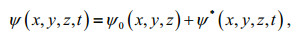 (5)
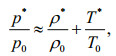
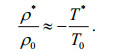
(5)where ψ*≪ψ0, with ψ represents absolute temperature T, pressure p and density ρ.
The equation of state
 (6)
(6)can be written as
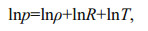 (7)
(7)where R=8.314 41±0.000 26 [J/mol.K] is the molar gas constant, to give
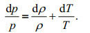 (8)
(8)Since
 (9)
(9)and
 (10)
(10)Eq.1 can be written as
 (11)
(11)where δ is the Kronecker delta.
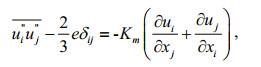
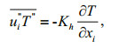
By applying a volume filter to the governing equations, those scales larger than the cutoff scale Δx are retained and classified as 'resolved scales', while scales smaller than the cutoff scale Δx are filtered, and classified as sub-grid scales. The filtered equation yields an additional term, which can be parameterized using an improved version of the 1.5-order closure from Moeng and Wyngaard (1988) and Saiki et al. (2000). Similar to the RANS model, PALM introduces eddy viscosities Km and Kh, and assumes that the secondary moments of the mean quantities are proportional to their gradients by
 (12)
(12) (13)
(13)and
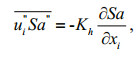 (14)
(14)where Km is the subgrid-scale eddy viscosity and Kh is the local subgrid-scale eddy diffusivity of heat. The viscosities can be parameterized as
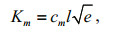 (15)
(15)and
 (16)
(16)where cm=0.1, Δ=
 (17)
(17)Here, ρθ is calculated by the method proposed by Jackett et al. (2006) using the polynomials determined by the variables Sa, θ and p (see Jackett et al., 2006, Table A2). Only the initial values of p are used here.
2.2 Initial conditionsThe size of the domain is 10.0 m×10.0 m×10.0 m, with a mesh resolution of 0.1 m×0.1 m×0.1 m. The potential temperature at the sea surface is set to 275 K, the vertical gradient for -5 m≤z≤0 is 1.5 K/100 m, and that for -10 m≤z≤-5 m is 1.0 K/100 m. The salinity at the sea surface is 32.0, with vertical gradients for -5 m≤ z≤0 and -10 m≤z≤-5 m of 1.5/100 m and 1.0 /100 m, respectively. The u-component of the background velocity is set to 1 m/s, with the v-component set to zero. The u-component of the geostrophic velocity at the surface is 1 m/s, while the v-component at the surface is zero. The Coriolis force is negligible, and the roughness length is 0.1 m.
2.3 Boundary conditionsThe upper boundary condition of the horizontal velocity components u and v follow the free-slip condition,
 (18)
(18) (19)
(19)where u and v are the horizontal components of the water velocity at the surface. The lower boundary condition of u and v follow the no-slip condition,
 (20)
(20)The lower boundary condition of the perturbation pressure is set as p(k=0)=0, and the upper boundary condition of the perturbation pressure is set as 
The lateral (streamwise and spanwise) boundary conditions are cyclic, with Dirichlet (inflow) and radiation (outflow) conditions allowed along the x- or y-direction.
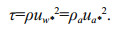
If the topography is described by a linear function, a singularity results at the top of the hill. To avoid this, while simulating a more realistic ocean-bed topography, the seabed is described by trigonometric functions. Calhoun and Street (2001) modeled turbulent flow over a wavy surface and showed that a recirculation region develops with the amplitude of the trigonometric function. Here, we investigate two cases with different topographies δ=0.75 and δ=0.2, where δ=2a/(λ/2) is the slope steepness, a is the amplitude of the wavy surface, and λ is the wavelength. The high hill topography is shown in Fig. 1, and is described by the function 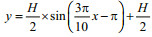


|
| Figure 1 High hill topography (H=5/2 m) at the seabed boundary |

|
| Figure 2 Low hill topography (H=2/3 m) at the seabed boundary The hill top is located at (5 m, -9.3 m), with sections s1–s5 consistent with Fig. 1. |
To discuss the TKE in different areas of the flow, and especially to compare the windward slope with the leeward slope of the hill (see Section 4.4), the hill topography is divided into five sections (s1, s2, s3, s4, s5) (Fig. 1).
The peak is located at (5 m, -7.5 m). The area is divided into five sections (s1–s5). Section s1 covers the area 1 m≤x≤2 m, s2 covers the area 3 m≤x≤4 m, s3 covers the area 4.5 m≤x≤5.5 m, s4 covers the area 6 m≤x≤7 m, and s5 covers the area 8 m≤x≤9 m. The sections represent the first valley (s1), windward slope (s2), peak (s3), leeward slope (s), and second valley (s5).
According to the early work of Jackson and Hunt (1975), the area over a two-dimensional wavy lower boundary can be divided into two regions: an inner region and an outer region. Similarly, in our model, the area over a three-dimensional wavy seabed boundary is divided into an inner region and an outer region, with the two regions having a different dimensionless height H. Here, we estimate the inner region depth as hi=H (Figs. 1 and 2). The TKE generated by the influence of the wave lower boundary cannot impact the outer region, while the lower hill produces the main turbulence shear in the inner region.
3 RESULTAccording to the normalization method of Kantha and Clayson (2004), the u-, v-, and w-components of the velocity can be normalized by uw* corresponding to the water-side friction velocity, and calculated as
 (21)
(21)Here, ua* is the atmosphere-side friction velocity, ρa is the air density, and τ is the shear stress, which can be calculated using the wind speed 10 m above the sea surface (u10) and the drag coefficient Cd,
 (22)
(22)where Cd is obtained from Wu (1980) as
 (23)
(23)Here we focus on the influence of the wavy seabed boundary. All velocity components have similar orders of magnitude because of the conservation of the whole water mass. Therefore, the water-side friction velocity uw* can normalize all velocity components.
The influence of the lower boundary on the turbulent statistics takes 1 200 s to reach a state of equilibrium.
3.1 u-component of the velocityAfter initialization, the numerical model integrates for 7 200 s (2 h). In the y-direction, the profiles of the u-component of the velocity at s1–s5 are captured at y=0.5 m, 3.5 m, 5.5 m, 7.5 m, and 10 m, with Fig. 3 showing these profiles after 1 200 s. The profiles at other times present almost identical values of the velocity, as well as velocity gradients, indicating that the model has attained a stable stage at this time.

|
| Figure 3 Depth profiles of the high hill model showing the u-component of the velocity at sections s1–s5 in the y-direction after 1 200 s for (a) y=0.5 m, (b) y=3.5 m, (c) y=5.5 m, (d) y=7.5 m, and (e) y=10.0 m The grey area represents the topography. The u-component of the velocity is normalized by the water-side friction velocity. |
In Fig. 3, each profile is divided into two parts. For -7 m≤z≤0, has a maximum of about 1.5 m/s near z= -3.5 m, and decreases toward the upper surface, as well as at -7 m, which is the height around the peak of the hill. For z≤-7 m, there is a countercurrent on the windward slope, with a maximum of about -0.5 m/s. On the leeward slope, the velocity is usually positive, with a maximum of about 0.5 m/s.
Furthermore, at z=-7 m, the vertical gradient of u is large, which implies that most of the TKE is generated in this area as a result of the shear induced by the topography. The area above the center of the trough is the maximum of the negative value, which implies high turbulence.
3.2 v-component of the velocityFigure 4 shows the profiles of the v-component of the velocity at sections s1–s5 after 1 200 s, indicating similar profiles at all five sections at this time, and thus a lack of variation of v in the y-direction.

|
| Figure 4 Depth profiles of the high hill model showing the v-component of the velocity at sections s1–s5 in the y-direction after 1 200 s for (a) y=0, (b) y=3 m, (c) y=5 m, (d) y=7 m, and (e) y=10 m The grey area represents the topography. The v-component of the velocity is normalized by the water-side friction velocity. |
At 1 200 s, there is a strong countercurrent on the windward slope of the middle hill (see Fig. 4) with a maximum v of about -0.9 m/s, while v above the countercurrent is positive and has a maximum of about 0.9 m/s. At z=-7 m, TKE production is strong, especially over the windward slope where the two opposite groups touch. The countercurrent in the area above the trough is still strong, showing a similar distribution pattern to that of u. Thus, the TKE over the windward slope is still strong.
3.3 w-component of the velocityFigure 5 shows the profiles of the w-component of the velocity at sections s1–s5 after 1 200 s, which is negative above the windward slope with a maximum of about -0.9 m/s, implying the flow descends beyond the middle hill. The velocity above the leeward slope is 0–0.5 m/s, indicating ascending flow in the area above the lee side. Figure 5 indicates that the profiles of w in the y-direction are similar to each other, as well as to v in the y-direction, thus demonstrating the conservation of water mass, such that any volume of water flowing upward, must be replaced by water moving downward, resulting in convective motion.

|
| Figure 5 Depth profiles of the high hill model showing the w-component of velocity at sections s1–s5 in the y-direction after 1 200 s for (a) y=0.5 m, (b) y=3.5 m, (c) y=5.5 m, (d) y=7.5 m, and (e) y=10 m The grey area represents the topography. The w-component of the velocity is normalized by the water-side friction velocity. |
The profiles clearly show two counteracting groups at the hill top above the valley, indicating a strong TKE at this location, which agrees with the experimental results reported in Poggi et al. (2007).
3.4 TKE budget 3.4.1 Horizontal average over the total model domainFollowing Eq.1, the horizontally-averaged subgrid-scale TKE equation after tensor contraction is
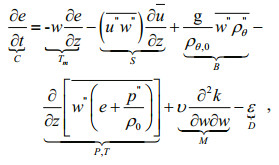 (24)
(24)where the quotation marks represent the subgrid-scale values and the overbars represent average values. Here, ρθ can be calculated from the state equation of seawater as proposed by Jackett et al. (2006), where ρθ depends on Sa, T and p (see Jackett et al., 2006, Table A2). For simplification, we set the value of ρθ as constant to 1.025 7×10³ kg/m3. On the right-hand side of Eq.24, the first term represents the mean velocity transport Tm, the second term represents the shear production S, the third term represents the buoyancy production B, the fourth and the fifth terms represent the pressure and turbulent transports denoted P and T, respectively, the sixth term represents the molecular viscosity diffusion M, and the last term represents the turbulent dissipation D. The term on the left-hand side of the equation is denoted C, and represents the time derivative of the subgrid-scale TKE. Here, the buoyancy production B is zero because of the constant density ρθ, and the molecular diffusion M is several orders of magnitude smaller than the other terms on the right-hand side, so that it may be ignored. While Calhoun and Street (2001) showed that Tm is a significant part of the TKE budget, our results show that the order of magnitude of Tm is less than 10-7 m2/s3, while the minimum value of the other terms is 10-7 m2/s3. Therefore, Tm has a smaller effect in this simulation. Equation 24 implies that the rate of change over time of the subgrid-scale TKE C is equal to the sum of the mean velocity transport Tm, the production S, the transport terms P and T, and the turbulent dissipation D.
As shown in Fig. 6, the subgrid-scale TKE remains almost constant in time, indicating that the rate of change of the subgrid-scale TKE with time is close to zero. Hence, the sum of the terms on the right-hand side of Eq.24 should also be close to zero. Indeed, in Fig. 6, for each horizontal sea layer, the sum of S, Tm, P, T, and D is approximately zero.

|
| Figure 6 High hill model depth profiles of TKE budget parameters for 1 800 s, 3 600 s, 5 400 s and 7 200 s after model initialization Solid blue line: shear production (S); dashed purple line: dissipation (D); dotted black line: mean velocity transport (Tm); dash-dotted red line: turbulence and pressure transport (P, T). |

|
| Figure 7 Low hill model depth profiles of the TKE budget parameters for 1 800 s, 3 600 s, 5 400 s, and 7 200 s Solid blue line: shear production (S); dashed purple line: dissipation (D); dotted black line: mean velocity transport (Tm); dash-dotted red line: turbulence and pressure transport (P, T). |
Close to the sea surface and z=-7.5 m (the top of the hills), S and D change suddenly, while P and T do not. Changes in the area close to the sea surface result from various factors acting at the sea surface, such as the wind stress, so that the shear stress produces TKE. At the same time, the topographic changes in the area above the hilltops also cause a shear and TKE production. In the area above the hilltops, the maximum rate of change in TKE is at the peak of the hill. The redistribution of production and dissipation results in a variation of P and T, resulting in changes to the transfer of energy.
3.4.2 Shear productionAs shown in Fig. 8, the simulation domain is divided into five sections (s1, s2, s3, s4, s5), with s1 covering the area 1 m≤x≤2 m, s2 the area 3 m≤x≤4 m, s3 the area 4.5 m≤x≤5.5 m, s4 the area 6 m≤x≤7 m, and s5 the area 8 m≤x≤9 m. The average is the horizontal average over each section, including the total domain average (s0). All the sections show a maximum at z=-7.5 m, with s3 having the highest value, indicating that the shear production is largest above the hilltop. Moreover, the shear production above the leeward slope is larger than that above the windward slope, indicating stronger turbulence above the leeward slope.

|
| Figure 8 Depth profile after 1 800 s comparing the shear production for different sections and in the total simulation domain s0 (total simulation domain, dark blue); s1 (1 m≤x≤2 m, red); s2 (3 m≤x≤4 m, yellow); s3 (4.5 m≤x≤5.5 m, purple); s4 (6 m≤x≤7 m, green), and s5 (8 m≤x≤9 m, light blue). |
As shown in Fig. 9, all the sections show peaks at z=-7.5 m, with s3 having the maximum value, indicating that the dissipation is largest above the hilltop. Thus, the turbulence dissipates rapidly in accordance with the slope of the topography. Moreover, the dissipation above the windward slope is smaller than that above the leeward slope, indicating reduced turbulence dissipation above the windward slope.

|
| Figure 9 Depth profile after 1 800 s Comparison of the dissipation between the different sections and the total simulation domain, with the sections (s0–s5) the same as in Fig. 8. |
Analysis of the turbulent kinetic energy produced by the LES model PALM allowed the influence of a wavy lower boundary on the redistribution of the TKE budget to be investigated. One of the first studies to investigate in detail the turbulent air flow over a low hill in the atmospheric boundary layer, Jackson and Hunt (1975) found that the maximum velocity occurs mostly in the area above the top of the hill, with the velocity over the upwind slope of the hill at the same elevation almost equal to that over the top of the hill. Although Jackson and Hunt (1975) used a low hill as the topography and some of their conclusions are similar to those of our study, their conclusions only apply to the atmospheric boundary layer. In 1994, the Coastal and Hydraulics Laboratory (formerly the Coastal Engineering Research Center) of the US Army Engineer Waterways Experiment Station performed a variety of laboratory experiments including those with different topographies (http://www.frf.usace.army.mil/duck94/DUCK94.stm). Their experiment, 'Sediment Dynamics in the Nearshore Environment', showed that (1) a wavy lower boundary can lead to higher water velocities, and (2) the velocity decays as the elevation rises. These conclusions are similar to our findings. Poggi et al. (2007) also investigated the distribution of the velocity field over a hilly surface, and simplified the filtered equations. Their results regarding the velocity field are similar to ours, although our analysis includes the influence of the wavy seabed boundary on the TKE budget redistribution.
We considered two different wavy boundaries with different relative hill height based on the steepness δ to distinguish the different hill heights (δ=0.75 and 0.2). As the hill height decreases, the resolution of the calculation needs to increase and, therefore, the requirements of the computational performance and time are higher, leading to higher costs. We found that, for a sufficiently low hill height, the influence of the wavy lower boundary on the TKE budget redistribution only slightly varies. It is worth noting that, apart from the shape and height of the hills, the tilt of the hills and the distance between two adjacent hills also affects the TKE budget redistribution.
5 CONCLUSIONAn LES model to simulate the influence of a wavy lower boundary allowed the analysis of the distribution of the velocity components and the redistribution of the TKE budget. The analysis of the distribution of the u-, v-, and w-components of the velocity shows that the flow over the center of the trough exhibits large velocity gradients, implying that the area over the center of the trough has a strong shear, leading to high TKE production.
The analysis of the redistribution of the TKE budget shows that, apart from the area close to the water surface where shear is produced by the complex sea-surface motion, the area above the seabed hilltops also produces turbulence. Our results show that shear production dominates the turbulent kinetic energy, although we have neglected buoyancy production here. The effect of the mean velocity transport is small. Furthermore, the shear production reaches a maximum above the hilltop and is larger above the leeward slope than above the windward slope.
Finally, the existence of a recirculation region (Calhoun and Street, 2001) over the trough is confirmed for different heights of the hill topography. Most of the TKE distribution occurs in the layer above the trough near the top of the hill, followed by in the recirculation region near the trough.
6 ACKNOWLEDGEMENTWe thank the two anonymous reviewers for their constructive comments.
Broglia R, Pascarelli A, Piomelli U. 2003. Large-eddy simulations of ducts with a free surface. Journal of Fluid Mechanics, 484: 223-253.
DOI:10.1017/S0022112003004257 |
Calhoun R J, Street R L. 2001. Turbulent flow over a wavy surface:neutral case. Journal of Geophysical Research:Oceans, 106(C5): 9 277-9 293.
DOI:10.1029/2000JC900133 |
Chang Y S, Scotti A. 2004. Modeling unsteady turbulent flows over ripples:Reynolds-averaged Navier-Stokes equations(RANS) versus large-eddy simulation (LES). Journal of Geophysical Research:Oceans, 109(C9): C09012.
|
Grigoriadis D G E, Balaras E, Dimas A A. 2013. Coherent structures in oscillating turbulent boundary layers over a fixed rippled bed. Flow, Turbulence and Combustion, 91(3): 565-585.
DOI:10.1007/s10494-013-9489-1 |
Grigoriadis D G E, Dimas A A, Balaras E. 2012. Large-eddy simulation of wave turbulent boundary layer over rippled bed. Coastal Engineering, 60: 174-189.
DOI:10.1016/j.coastaleng.2011.10.003 |
Harris J C, Grilli S T. 2012. A perturbation approach to large eddy simulation of wave-induced bottom boundary layer flows. International Journal for Numerical Methods in Fluids, 68(12): 1 574-1 604.
DOI:10.1002/fld.v68.12 |
Henn D S, Sykes R I. 1999. Large-eddy simulation of flow over wavy surfaces. Journal of Fluid Mechanics, 383: 75-112.
DOI:10.1017/S0022112098003723 |
Jackett D R, McDougall T J, Feistel R, et al. 2006. Algorithms for density, potential temperature, conservative temperature, and the freezing temperature of seawater. Journal of Atmospheric and Oceanic Technology, 23(12): 1 706-1 728.
|
Jackson P S, Hunt J C R. 1975. Turbulent wind flow over a low hill. Quarterly Journal of the Royal Meteorological Society, 101(430): 929-955.
DOI:10.1002/(ISSN)1477-870X |
Kantha L H, Clayson C A. 2004. On the effect of surface gravity waves on mixing in the oceanic mixed layer. Ocean Modelling, 6(2): 101-124.
DOI:10.1016/S1463-5003(02)00062-8 |
Large W G, Gent P R. 1999. Validation of vertical mixing in an equatorial ocean model using large eddy simulations and observations. Journal of Physical Oceanography, 29(3): 449-464.
DOI:10.1175/1520-0485(1999)029<0449:VOVMIA>2.0.CO;2 |
Large W G, McWilliams J C, Doney S C. 1994. Oceanic vertical mixing:a review and a model with a nonlocal boundary layer parameterization. Reviews of Geophysics, 32(4): 363-403.
DOI:10.1029/94RG01872 |
Li M, Zhong L J, Boicourt W C. 2005. Simulations of Chesapeake Bay estuary:sensitivity to turbulence mixing parameterizations and comparison with observations. Journal of Geophysical Research:Oceans, 110(C12): C12004.
DOI:10.1029/2004JC002585 |
Li S, Song J B, He H L, et al. 2013. Large eddy simulation of turbulence in ocean surface boundary layer at Zhangzi Island offshore. Acta Oceanologica Sinica, 32(7): 8-13.
DOI:10.1007/s13131-013-0326-0 |
Li Y J, Chen J B, Zhou J F, et al. 2016. Large eddy simulation of boundary layer flow under cnoidal waves. Acta Mechanica Sinica, 32(1): 22-37.
DOI:10.1007/s10409-015-0486-6 |
Maronga B, Gryschka M, Heinze R, et al. 2015. The Parallelized Large-Eddy Simulation Model (PALM) version 4.0 for atmospheric and oceanic flows:model formulation, recent developments, and future perspectives. Geoscientific Model Development, 8(8): 2 515-2 551.
|
McWilliams J C, Sullivan P P. 2000. Vertical mixing by Langmuir circulations. Spill Science & Technology Bulletin, 6(3-4): 225-237.
|
Mellor G L, Yamada T. 1982. Development of a turbulence closure model for geophysical fluid problems. Reviews of Geophysics, 20(4): 851-875.
DOI:10.1029/RG020i004p00851 |
Moeng C H, Wyngaard J C. 1988. Spectral analysis of largeeddy simulations of the convective boundary layer. Journal of the Atmospheric Sciences, 45(23): 3 573-3 587.
DOI:10.1175/1520-0469(1988)045<3573:SAOLES>2.0.CO;2 |
Poggi D, Katul G G, Albertson J D, et al. 2007. An experimental investigation of turbulent flows over a hilly surface. Physics of Fluids, 19(3): 036601.
DOI:10.1063/1.2565528 |
Saiki E M, Moeng C H, Sullivan P P. 2000. Large-eddy simulation of the stably stratified planetary boundary layer. Boundary-Layer Meteorology, 95(1): 1-30.
DOI:10.1023/A:1002428223156 |
Smyth W D, Skyllingstad E D, Crawford G B, et al. 2002. Nonlocal fluxes and Stokes drift effects in the K-profile parameterization. Ocean Dynamics, 52(3): 104-115.
DOI:10.1007/s10236-002-0012-9 |
Soldati A, Marchioli C. 2012. Sediment transport in steady turbulent boundary layers:potentials, limitations, and perspectives for Lagrangian tracking in DNS and LES. Advances in Water Resources, 48: 18-30.
DOI:10.1016/j.advwatres.2012.05.011 |
Umlauf L, Burchard H. 2003. A generic length-scale equation for geophysical turbulence models. Journal of Marine Research, 61(2): 235-265.
DOI:10.1357/002224003322005087 |
Walker R, Tejada-Martínez A E, Grosch C E. 2016. Largeeddy simulation of a coastal ocean under the combined effects of surface heat fluxes and full-depth Langmuir circulation. Journal of Physical Oceanography, 46(8): 2 411-2 436.
DOI:10.1175/JPO-D-15-0168.1 |
Wijesekera H W, Allen J S, Newberger P A. 2003. Modeling study of turbulent mixing over the continental shelf:comparison of turbulent closure schemes. Journal of Geophysical Research:Oceans, 108(C3): 3103.
DOI:10.1029/2001JC001234 |
Wilcox D C. 1988. Reassessment of the scale-determining equation for advanced turbulence models. AIAA Journal, 26(11): 1 299-1 310.
DOI:10.2514/3.10041 |
Wu J. 1980. Wind-Stress coefficients over sea surface near Neutral Conditions-a revisit. Journal of Physical Oceanography, 10(5): 727-740.
DOI:10.1175/1520-0485(1980)010<0727:WSCOSS>2.0.CO;2 |
Zeng J, Constantinescu G, Blanckaert K, et al. 2008. Flow and bathymetry in sharp open-channel bends:experiments and predictions. Water Resources Research, 44(9): W09401.
|