 2018, Vol. 36
Institute of Oceanology, Chinese Academy of Sciences
Article Information
- ZHANG Xin(张新), LIU Yuqi(刘玉琦), CHEN Yongxin(陈永新)
- Development of a location-weighted landscape contrast index based on the minimum hydrological response unit
- Chinese Journal of Oceanology and Limnology, 36(4): 1236-1243
- http://dx.doi.org/10.1007/s00343-018-7069-x
Article History
- Received Mar. 12, 2017
- accepted in principle Jun. 9, 2017
- accepted for publication Jul. 3, 2017


2 University of Chinese Academy of Sciences, Beijing 100049, China
Water is the source of life and essential for human survival. However, human activities, such as deforestation and excessive fertilization, have resulted in damage to ecosystems that inevitably changes the original pattern of river basin landscapes. These changes cause a high degree of non-point source pollution via surface runoff and groundwater migration and pose a threat to both aquatic ecosystems and human health. The study of the hydrological response to landscape patterns has been the focus of watershed ecological research. In complex ecological river basin systems, ecological processes are interrelated in terms of their geographical location, biological processes and physical environment, such that the damage from agricultural non-point source pollutants to the aquatic environment in the watershed is also characterized by complex relationships. From the perspective of non-point source pollution, landscape pattern plays an important role in the process of pollutant spread (Verburg et al., 2009).
The advantages of remote sensing data, including that they are multiphase and multiresolution and allow large-scale synchronous observation, make them the main data source used to study the landscape pattern (Fichera et al., 2012). Accurately extracting feature-type information from remote sensing data facilitates the next step of computing the source of landscape pattern information (Chen et al., 2012). The use of remote sensing and GIS techniques to analyze landscape pattern is the basis for studying the relationship between pattern and ecological processes and is key to the study of landscape dynamics and function (Yang and Liu, 2005). In addition, landscape pattern analysis plays an important role in resource management and biodiversity. For these reasons, the study of landscape pattern analysis has been an ongoing effort (Wang et al., 2009). Remote sensing data are used to obtain landscape pattern information (Yang, 2005; Yu and Ng, 2006), which can be used to calculate the spatial load of non-point source pollution.
To extract landscape pattern information, Chen et al. (2003) proposed a location-weighted landscape contrast index (LCI) that links the landscape pattern with non-point source pollution processes and enables the quantitative study of the relationship between landscape pattern and ecological processes. Based on a spatial load contrast index, a grid landscape contrast index (GLCI) was constructed by Jiang et al. (2013).
In this paper, an ecological landscape spatial load contrast index was constructed, the results of which reflect the contribution of the region to non-point source pollution. Compared to traditional landscape indices, the new index in this paper takes into account the effect of research scale. Combined with the process of non-point source pollution, the calculation results of the index can effectively reflect the contribution difference made by 'source' and 'sink' regions to non-point source pollution loads in the watershed landscape pattern. Therefore, this landscape index is characterized by its ecological focus and multiple scales. This paper describes the effect of landscape pattern on the non-point source pollution process from the minimum hydrological response unit (HRU).
2 MATERIAL AND METHOD 2.1 Research area and data sourceThe Yanshi River runs through Yanshi town within Longyan city in Fujian Province (24°55′–25°21′N, 116°49′–117°14′E) and is one of the upstream tributaries of the Jiulong River (Fig. 1), with a drainage area of 1 459 km2. The Yanshi River originates in the Longmen River, and the trunk stream length is 96.5 km. The average annual flow is 47.72 m3, and the average annual runoff is 1.505 billion m3. The gradient of 24.2 m per thousand meters allows the development of hydropower resources with an installed capacity of 30 800 kilowatts. The three main tributaries of the Yanshi River are Longmen Creek (Xiaochi Creek), Dongbang Creek (Xiao Creek) and Feng Creek, and these three main tributaries converge in the city.

|
| Figure 1 Location of the Yanshi River Basin |
The data used in the calculation of the minimum hydrological response unit (HRULCI) included 2014 remote sensing image data from GF-2 (available from China Centre for Resources Satellite Data and Application), Digital elevation model data (Fig. 2) (available from the U.S. Geological Survey), 1:1 million Chinese soil texture data (available from Harmonized World Soil Database), 2014 precipitation data (available from China Meteorological Data Service Center), and statistical yearbook data. The land use/cover data are based on high resolution remote sensing image data of GF-2 for the Yanshi River watershed. According to the national land use classification standards, there are many types of land use/cover change (LUCC) in the Yanshi River basin, such as cultivated land, plant, shrub land, orchard, rivers, lakes, construction land, forest, wetland and unused land. The soil types in the basin are red soil, paddy soil, purple soil, and yellow soil. Average precipitation data for 2014 were obtained from the Chinese meteorological data monitoring station.

|
| Figure 2 Remote sensing image of GF-2 satellite and digital elevation model (DEM) (measured in meters) of the Yanshi River in 2014 |
Dividing the HRU: The minimum hydrological response unit of the basin reflects a relatively homogeneous area of the underlying soil surface (Kumar and Mishra, 2015). In traditional locationweighted landscape contrast index calculation, the smallest unit of research is chosen by dividing the landscape arbitrarily into grid cells. Although this method is convenient for grid data processing, its flaw is that there is no scientific basis for the individual units. Indeed, there is a relationship between the landscape pattern and geographical factors, which the mandatory division of the grid divides (Sun et al., 2012). There is also a scale effect on the relationship between the landscape pattern and ecological processes, and discussion is needed as to whether the fixed size grid unit is the most appropriate scale unit. Compared with the artificial division of the grid unit, the smallest research unit selection of HRU forms a sounder ecological base.
When the traditional landscape index is used to evaluate the landscape pattern, the result is often a numerical calculation (Chen et al., 2003). For example, remote sensing indices (Normalized Difference Vegetation Index, Leaf Area Index) describe the overall landscape with a single numerical result, and the internal differences of the landscape pattern are neglected. Thus, when the internal landscape changes, the traditional landscape index calculation results may not reflect these changes (Lausch and Herzog, 2002). Therefore, this paper proposes a location-weighted landscape contrast index, which needs to meet the following three requirements: (1) remote sensing data is the underlying data, so the calculation method of the new index should be consistent with the processing mode for raster data; (2) the HRULCI should be of ecological significance and reflect the relationship between the landscape pattern and non-point source pollution; and 3) the results of the HRULCI should reflect the spatial differences in the regional contribution of non-point source pollution between different regions, that is, the spatial heterogeneity.
Determination of the geographical correction factor: Different geographical factors play different roles in non-point source pollution. Taking annual precipitation as an example, higher annual precipitation will lead to a greater possibility of surface runoff, accompanied by soil erosion and nutrient loss. Therefore, precipitation contributes positively to the process of non-point pollution (Herzog et al., 2001). In contrast, NDVI reflects the surface vegetation biomass: compared with bare land, forest conserves soil and water better, so vegetation has a negative effect on non-point pollution (Emili and Greene, 2013).
There are two key points in the calculation of HRULCI: the first is selecting the appropriate geographical variables. In this paper, the selection of factors was based on the principle of being comprehensive and independent, that is, considering the geographical factors as much as possible and ensuring that they have a weak correlation (Griffith, 2002). The second is to determine the correction factor for geographical variables. In this paper, with reference to the standard Chinese farmland pollutant runoff discharge coefficient, we used the paddy field both as the reference standard and to revise the influencing factors (Herzog and Lausch, 2001).
2.2.1 Division of HRURemote sensing image data from GF-2 were the basic data used to extract the watershed landscape information. In this paper, to obtain high-precision data after classification, artificial visual interpretation was used to classify 2014 land use data (Fig. 3; Table 1). Soil information was obtained from the 1:100 million Chinese soil texture data.

|
| Figure 3 Landscape pattern in the Yanshi River region in 2014 |

ArcGIS (ESRI, Redlands, CA) was used to extract sub-basin information from DEM data, and the data were analyzed by spatial statistical superposition analysis using landscape source and sink, and soil distribution data. The sub-watershed was divided into a plurality of HRUs with only a single land use type and a soil type (Liu et al., 2013), and the spatial distribution characteristics of the underlying surface factors were represented in the form of discretization. Efficiently and accurately extracting the river basin DEM is the focus of the software in the hydrological analysis module, so by setting different thresholds and comparing the division of the river water and river basin differences to determine the final threshold size, we obtained a reasonable distribution of the drainage network data (Pietroniro et al., 1996). We superimposed an analysis of spatial data to determine the watershed HRU division results. We used conditions settings to merge very small HRUs into larger HRUs (Zehe et al., 2014).
There were 638 HRUs in the Yanshi River Basin with a single type of land use and soil type in each hydrological unit (Fig. 4), which reflected not only the spatial heterogeneity of the underlying basin surface but also the internal homogeneity of each research unit of LUCC and soil type (Zhang et al., 2009).

|
| Figure 4 The hydrological response units (HRUs) of the Yanshi River region in 2014 |
Taking into consideration the influence of geographical factors in the process of non-point source pollution transmission in the watershed, effective soil moisture, soil texture, slope, land use types, annual precipitation, the effective distance and NDVI were selected as influencing factors (Jiang et al., 2013).
The effective soil moisture and soil texture characterize the soil properties in the watershed, mainly reflecting the effect of soil on surface runoff. The slope represents terrain information in the watershed. The type of land use is the basis for distinguishing the source and sink landscapes, bearing in mind that the intensity of different source (or sink) landscapes on the non-point source pollutant diffusion process is variable. The annual average rainfall is an important measure of climate in the study area. Under the same surface conditions, the erosion intensity of rain affects the effective transmission of non-point source pollutants. NDVI reflects the amount of surface vegetation and the conservation capacity of soil and water tends to be stronger where the value of NDVI is high.
With reference to the Chinese standard farmland runoff pollutants discharge coefficient and according to the actual situation in the Yanshi River in 2014, we used the paddy field as the reference standard and to revise the influencing factors.
The definition and correction coefficient for standard farmland: standard farmland includes a plains landform, planted with wheat, with a loam soil. Chemical fertilizer is applied at the rate of 151.757– 212.460 kg/acre/year, and precipitation is in the range of 400–800 mm.
(1) Slope correction (Fig. 5). When the slope of the land was below 25 degrees, the loss coefficient was 1.0–1.2; when the slope was greater than 25 degrees, the loss coefficient was 1.2–1.5.

|
| Figure 5 Distance and slope of the Yanshi River region in 2014 |
(2) Crop type correction. According to the actual situation of the Yanshi River, this paper provided different correction coefficients for forest and shrub land, cultivated land and orchard, and other cases. The correction coefficient for forest and shrub land was 0.7, and the correction coefficient for cultivated land and orchard was approximately 1, and the other modified coefficient was approximately 1.5.
(3) Soil type correction. The soil in the Yanshi River basin is classed by its texture, which is the ratio of clay and sand in the soil composition and is divided into sand, loam and clay. The correction coefficient for loam was 1, the correction coefficient for sandy soil was 0.8–1.0, and the correction coefficient for clay was 0.6–0.8.
(4) Chemical fertilizer amendment correction. If the amount of chemical fertilizer per mu was below 25 kg, the correction coefficient was 0.8–1.0; if the amount was between 25 and 35 kg, the correction coefficient was 1.0–1.2; and if the amount was more than 35 kg, the correction coefficient was 1.2–1.5. The Yanshi River basin is located in Xinluo County of Longyan City, Fujian Province. According to the statistical yearbook, in 2014, the amount of chemical fertilizer used in farmland and orchard was approximately 250.4 kg/acre/year; therefore, the correction coefficient of cultivated land and orchard was 1.4, and that for other surface types was 0.8.
(5) Precipitation correction. The correction coefficient for annual precipitation below 400 mm was 0.6–1.0; the area correction coefficient for annual precipitation between 400 mm and 800 mm was 1.0– 1.2; and the correction coefficient for annual precipitation above 800 mm was 1.2–1.5.
(6) NDVI correction. The reason why NDVI is an influencing factor is that NDVI can reflect the difference in vegetation biomass information. In the case of forest, tree density differs across regions, necessitating the use of NDVI to reflect the biomass of different regions.
(7) Effective distance correction (Fig. 5). The farther away from the water body, the less likely it is that the non-point source pollutant will enter it. We used the 20 km maximum for local water source protection as the most effective surface distance. The distance from the water body was used to determine the correction factor.
(8) Available Water Content (AWC) of soil correction. AWC represented the water in soil that can be absorbed by crop water, namely, the field moisture between field water capacity and the wilting coefficient. The soil suction force was related to the available soil water content, such that, all other conditions being equal, the greater the soil moisture, the smaller the soil suction, and the more effective the water content.
3 RESULT AND DISCUSSION 3.1 Calculation of HRULCITo study the landscape pattern, the landscape index must be ecologically significant. To characterize specific ecological processes, such as non-point source pollution, the landscape index must reflect the links between the landscape pattern and non-point source pollution. The HRULCI describes this relationship in the watershed, and the results show the influence of different areas in the watershed landscape on non-point source pollution.
Based on HRU, the calculation formula of the location-weighted landscape contrast index is expressed as
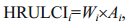 (1)
(1)where i refers to a specific HRUi, Ai is the area of HRUi, and Wi is the weight of emission of a pollutant from a given source or sink landscape type that is affected by land use, soil properties, precipitation and fertilizer application. When considering the process of non-point source pollution from HRU production or attenuation and final entry into the water body, it is necessary to revise the different geographical factors, so Wi can be expressed as
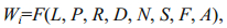 (2)
(2)where L refers to LUCC correction, P refers to slope correction, R refers to precipitation correction, D refers to effective distance correction, N refers to NDVI correction, S refers to soil type correction, F refers to chemical fertilizer amendment correction, and A refers to the AWC of soil correction.
At the same time, to compare the different HRULCI, the pollutant correction coefficients for different landscape source sink types need to be standardized:
 (3)
(3)where Wi refers to a non-point source pollutant correction factor for a land use landscape and WMAX is the maximum value of the non-point source pollutant correction coefficient in the watershed landscape. Considering the existence of various types of pollutants, HRULCI can be expressed as
 (4)
(4)where HRULCIY refers to the HRULCI of non-point source pollutant Y and HRULCIXY is the HRULCI of sum of X and Y.
For the sub-basin, the non-point source pollution location-weighted landscape contrast index is calculated as
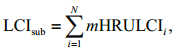 (5)
(5)where N refers to the number of HRU in sub-basin and i refers to HRU. Comparing the LCIsub between different sub-basins, larger LCIsub values lead to a stronger relative effect of the sub-basin on non-point source pollution, greater risk of nutrient loss and greater propagation of non-point source pollutants. After calculating the HRULCI of the time series, we can compare the numerical changes of different regions to reflect the changes in non-point source pollution over multiple years. The lower the numerical value, the greater is the improvement in the landscape source and sink pattern, and vice versa.
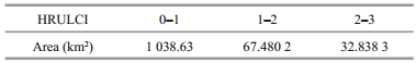
The HRULCI calculation result of Yanshi River basin is shown in Fig. 6 and Table 2.

|
| Figure 6 HRULCI of the Yanshi River region in 2014 |
|
(1) The HRULCI results for the Yanshi River show that numerically higher areas were concentrated in the cultivated lands. The reason was that cultivated land had less vegetation cover, and the soil texture was loose; therefore, the soil erosion and nutrient loss on cultivated land were more significant. Further, cultivated land usually included artificial fertilization, which indicated that it played an important role in promoting agricultural non-point source pollution. The results show that the mid-range values were concentrated in the residential lands and orchards. In residential land, the vegetation coverage rate was low, and the surface was impervious to water. Although the phenomena of soil erosion and nutrient loss were not obvious, residents produced a great deal of nonpoint source pollutants, so the HRULCI value was second only to that of cultivated land. Compared with cultivated land, the soil in orchard areas was harder, and the soil and water conservation of the fruit trees was higher than that of the crops, leading to values slightly lower than for cultivated land. The above two land use types had HRULCI values higher than 1, indicating that they promoted transport of non-point source pollutants. Higher values show a more obvious promotion effect. The lowest HRULCI values were obtained in forest and shrub forest areas. Because of the high vegetation coverage in these areas, they had a strong ability to conserve water and soil. In this case, the HRULCI value was less than 1, which indicated that they inhibited non-point source pollutant transport. Smaller values equate to greater inhibition.
(2) After calculation, HRULCI can be used to calculate the relative degree of contribution of nonpoint source pollution, which is of great significance to its prevention and control. On the one hand, regions with a large contribution should be key control areas, and reducing the size of such areas can effectively reduce non-point source pollution. On the other hand, by monitoring the change over a certain period of time, we can monitor the change in the landscape source and sink pattern within the watershed. If the value increases, it would indicate that the source landscape had become the dominant landscape and vice versa, and this could be the basis of efforts to study the landscape and predict further changes.
(3) The traditional dynamic monitoring of the landscape pattern is often from the perspective of land use change detection by analyzing the landscape pattern changes over a certain period of time through the conversion of surface types. This analytical method is characterized by easy-to-monitor landscape changes, but its disadvantage is that it is not associated with the underlying ecological processes. The superficial analysis of a change of surface type is insufficient to measure the ecological effects on the landscape. In this paper, by constructing HRU, the landscape pattern was related to the ecological processes affecting non-point source pollution, making the new index more ecologically relevant. The next step of the work will be to measure the landscape pattern changes in the Yanshi River Basin by comparing the changes in HRULCI over the years, from the aspect of non-point source pollution.
4 CONCLUSIONIn this paper, we proposed an improved locationweighted landscape contrast index. The newly established index has several beneficial characteristics. Compared with the artificial division grid unit with a fixed size, using the minimum HRU as the research unit has advantages. For example, while the land use and soil types are homogeneous in the same HRU, there are discrepancies among different HRUs, which can effectively reflect landscape heterogeneity. In the research of landscape pattern, we should pay attention to the scale effect and should verify whether a fixed size arbitrary grid unit is appropriate for the research. According to the first law of geography, all attribute values on a geographic surface are related to each other; this relativity may be damaged when researchers take a grid unit as the minimum research scale, because the same geographical object may be divided into two or more units. However, when we use the minimum hydrological response unit instead of the grid unit as the minimum research scale, this uncertainty can be avoided. HRULCI combines landscape pattern research and non-point source pollution processes, which makes the research more ecologically relevant and significant. Although the results of index calculation cannot be used to quantify the spatial load of non-point source pollution, the qualitative analysis of the contribution of different regions to non-point pollution is still significant for watershed pollution control.
5 DATA AVAILABILITY STATEMENTThe datasets generated and/or analyzed during the current study are available from the corresponding author on reasonable request.
6 ACKNOWLEDGEMENThe authors would like to thank the anonymous reviewers for their constructive comments and suggestions.
Chen G, Hay G J, Carvalho L M T, Wulder M A. 2012. Objectbased change detection. International Journal of Remote Sensing, 33(14): 4434-4457.
DOI:10.1080/01431161.2011.648285 |
Chen L D, Fu B J, Xu J Y, Gong J. 2003. Location-weighted landscape contrast index:a scale independent approach for landscape pattern evaluation based on "Source-Sink" ecological processes. Acta Ecologica Sinica, 23(11): 2406-2413.
(in Chinese with English abstract) |
Emili L A, Greene R P. 2013. Modeling agricultural nonpoint source pollution using a geographic information system approach. Environmental Management, 51(1): 70-95.
DOI:10.1007/s00267-012-9940-4 |
Fichera C R, Modica G, Pollino M. 2012. Land Cover classification and change-detection analysis using multitemporal remote sensed imagery and landscape metrics. European Journal of Remote Sensing, 45(1): 1-18.
DOI:10.5721/EuJRS20124501 |
Griffith J A. 2002. Geographic techniques and recent applications of remote sensing to landscape-water quality studies. Water, Air, and Soil Pollution, 138(1-4): 181-197.
|
Herzog F, Lausch A, Müller E, Thulke H H, Steinhardt U, Lehmann S. 2001. Landscape metrics for assessment of landscape destruction and rehabilitation. Environmental Management, 27(1): 91-107.
DOI:10.1007/s002670010136 |
Herzog F, Lausch A. 2001. Supplementing land-use statistics with landscape metrics:some methodological considerations. Environmental Monitoring and Assessment, 72(1): 37-50.
DOI:10.1023/A:1011949704308 |
Jiang M Z, Chen H Y, Chen Q H. 2013. A method to analyze "source-sink" structure of non-point source pollution based on remote sensing technology. Environmental Pollution, 182: 135-140.
DOI:10.1016/j.envpol.2013.07.006 |
Kumar S, Mishra A. 2015. Critical erosion area identification based on hydrological response unit level for effective sedimentation control in a river basin. Water Resources Management, 29(6): 1749-1765.
DOI:10.1007/s11269-014-0909-3 |
Lausch A, Herzog F. 2002. Applicability of landscape metrics for the monitoring of landscape change:issues of scale, resolution and interpretability. Ecological Indicators, 2(1-2): 3-15.
DOI:10.1016/S1470-160X(02)00053-5 |
Liu D L, Hao S L, Liu X Z, Li B C, He S F, Warrington D N. 2013. Effects of land use classification on landscape metrics based on remote sensing and GIS. Environmental Earth Sciences, 68(8): 2229-2237.
DOI:10.1007/s12665-012-1905-7 |
Pietroniro A, Prowse T, Hamlin L, Kouwen N, Soulis R. 1996. Application of a grouped response unit hydrological model to a northern wetland region. Hydrological Processes, 10(10): 1245-1261.
DOI:10.1002/(ISSN)1099-1085 |
Sun R H, Chen L D, Wang W, Wang Z M. 2012. Correlating landscape pattern with total nitrogen concentration using a location-weighted sink-source landscape index in the Haihe River Basin, China. Environment Science, 33(6): 1784-1788.
(in Chinese with English abstract) |
Verburg P H, Van De Steeg J, Veldkamp A, Willemen L. 2009. From land cover change to land function dynamics:a major challenge to improve land characterization. Journal of Environmental Management, 90(3): 1327-1335.
DOI:10.1016/j.jenvman.2008.08.005 |
Wang K, Franklin S E, Guo X L, He Y H, McDermid G J. 2009. Problems in remote sensing of landscapes and habitats. Progress in Physical Geography, 33(6): 747-768.
DOI:10.1177/0309133309350121 |
Yang X J, Liu Z. 2005. Quantifying landscape pattern and its change in an estuarine watershed using satellite imagery and landscape metrics. International Journal of Remote Sensing, 26(23): 5297-5323.
DOI:10.1080/01431160500219273 |
Yang X J. 2005. Remote sensing and GIS applications for estuarine ecosystem analysis:an overview. International Journal of Remote Sensing, 26(23): 5347-5356.
DOI:10.1080/01431160500219406 |
Yu X, Ng C. 2006. An integrated evaluation of landscape change using remote sensing and landscape metrics:a case study of Panyu, Guangzhou. International Journal of Remote Sensing, 27(6): 1075-1092.
DOI:10.1080/01431160500377162 |
Zehe E, Ehret E, Pfister L, Blume T, Schröder B, Westhoff M, Jackisch C, Schymanski S J, Weiler M, Schulz K, Allroggen N, Tronicke, van Schaik L, Dietrich P, Scherer U, Eccard J, Wulfmeyer V, Kleidon A. 2014. HESS Opinions:from response units to functional units:a thermodynamic reinterpretation of the HRU concept to link spatial organization and functioning of intermediate scale catchments. Hydrology and Earth System Sciences, 18(11): 4635-4655.
DOI:10.5194/hess-18-4635-2014 |
Zhang X, Jiang W G, Zhou Y G, Tang H. 2009. Hydrological response unit division for Dongting Lake based on DEM and GIS. Geography and Geo-Information Science, 25(4): 17-21.
(in Chinese with English abstract) |