 2019, Vol. 37
Institute of Oceanology, Chinese Academy of Sciences
Article Information
- WANG Yunhe, BI Haibo, HUANG Haijun, LIU Yanxia, LIU Yilin, LIANG Xi, FU Min, ZHANG Zehua
- Satellite-observed trends in the Arctic sea ice concentration for the period 1979-2016
- Journal of Oceanology and Limnology, 37(1): 18-37
- http://dx.doi.org/10.1007/s00343-019-7284-0
Article History
- Received Oct. 11, 2017
- accepted in principle Nov. 28, 2017
- accepted for publication Apr. 8, 2018


2 University of Chinese Academy of Sciences, Beijing 100049, China;
3 Laboratory for Marine Geology, Qingdao National Laboratory for Marine Science and Technology, Qingdao 266200, China;
4 College of Earth Science and Engineering, Shandong University of Science and Technology, Qingdao 266590, China;
5 Key Laboratory of Research on Marine Hazards Forecasting, National Marine Environmental Forecasting Center, Beijing 100081, China
Sea ice is an essential component of the climate system at high latitudes (Laxon et al., 2013; Zhai et al., 2015). It influences the weather and climate patterns at both the regional and global scales (Heygster et al., 2012; Overland et al., 2015). It serves as a sensitive indicator for changes in the global climate system and a diagnostic parameter for climate variations (Screen and Simmonds, 2010; Screen et al., 2015; Liu et al., 2016a, b). Normally, the albedo of sea ice is greater than 0.6 while that of water ranges from 0 to 0.07 (Perovich et al., 2007; Kharbouche and Muller, 2017). Therefore, sea ice is an efficient insulator that reflects solar radiation back to the sky, blocks wind from blowing over the sea, and reduces the fluxes of heat, momentum and water vapor between the ocean and the atmosphere (Lüpkes et al., 2008; Tschudi et al., 2008; Zhan and Davies, 2017). As a result, changes in Arctic sea ice play an important role in modulating the atmospheric and oceanic circulation modes (Liu et al., 2004; Ding et al., 2017).
Over the past few decades, increases in greenhouse gases within the atmosphere have contributed to the advancement of global warming (Mei et al., 2012). Moreover, the Arctic areas have been warming at a faster rate, corresponding to about two times the global average (Comiso, 2012), and possibly leading to a further extensive sea ice melting (Perovich and Richter-Menge, 2009; Ruckert et al., 2016). Therefore, thinner and younger sea ice cover components are highly expected in the Arctic Ocean in the near future (Maslanik et al., 2007b, 2011; Kwok et al., 2009).The physical mechanisms underlying the Arctic sea ice decline are complex, affected by both dynamical and thermodynamic processes. Existing investigations of the declining Arctic sea ice extent have analyzed the influences of different climate processes on the Arctic sea ice variations in terms of atmospheric and oceanic heat transport, air temperature, and the radiative effects of clouds (Francis and Hunter, 2006, 2007; Serreze et al., 2007; Liu et al., 2009; Liu and Schweiger, 2017). In addition, multiple studies have examined the changes in Arctic sea ice extent/area associated with the Arctic Oscillation (AO), North Atlantic Oscillation (NAO), Dipole anomaly (DA) (Kwok, 2000; Wang and Ikeda, 2000; Jung and Hilmer, 2001; Rigor et al., 2002; Holland, 2003; Wu et al., 2006; Seierstad and Bader, 2009; Strong et al., 2009), surface air temperature (SAT), sea surface temperature (SST), and atmospheric circulation patterns (Rayner et al., 2003; Liu et al., 2004; Gerdes, 2006; Zhao et al., 2006; Serreze et al., 2007; Holl and Stroeve, 2011; Comiso, 2012; Stroeve et al., 2012; Comiso and Hall, 2014; Ding et al., 2017). However, current studies mostly document a relatively shorterterm or single-case report for the feedbacks between climate changes and sea ice concentration (SIC). For example, some case studies assess the influences or feedbacks of substantial ice loss on the air temperature (Screen and Simmonds, 2010), clouds (Liu et al., 2004; Kay et al., 2008; Sedlar and Tjernström, 2017) and winds (Comiso et al., 2008), and SST anomalies in line with ice losses observed in the Pacific sector of the Arctic Ocean in the summers of 2007 (Perovich et al., 2008) and 2012 (Parkinson and Comiso, 2013).
To our knowledge, relatively few studies of longterm sea ice change from the perspective of SIC trends over different seasons and regions have been published. Comiso et al. (2008) examined the SIC trend in the Arctic Ocean for the period 1979–2006, while Parkinson and Cavalieri (2012) extended their time series to 2010. In addition, Stroeve et al. (2012) investigated the SIC trend only for the ice cover in September (1979–2012). More recently, Comiso and Hall (2014) discussed the SIC trend in the Arctic Ocean for the period 1979–2012 and reviewed its possible effects on the ocean/land surface temperature, snow cover, Greenland ice sheet, and landside permafrost temperature. However, the causes and feedbacks of SIC trends associated with the SAT, SST, and surface winds over the Arctic Ocean were not discussed despite the broad importance and interests represented by the changes in these parameters among the community studying climate change.
One of the objectives of this study is to investigate the spatiotemporal trends of the SIC in the Arctic Ocean over a longer period of 38 years (1979–2016). We also aim to examine the correlations between the SIC with the AO, NAO, DA, SAT, SST, and surface wind (SW) fields. This study is organized as follows. The data and methodology are described in Section 2. The SIC trends for the different seas in the Arctic Ocean are presented in Section 3. The coupled relationships between the SIC trends and the climate indexes and climatic parameters are analyzed in Section 4, and our concluding remarks are given in Section 5.
2 DATA AND METHODOLOGY 2.1 Data 2.1.1 SICPassive microwave sensors have provided a successive source of information about polar sea ice changes since October 1978. The monthly mean SIC data for the period from January 1979 to December 2016 was obtained from the National Snow and Ice Data Center (NSIDC, http://nsidc.org/data/NSIDC-0051) and mapped onto a polar stereographic projection with a grid cell size of 25 km×25 km. These data are derived from multiple satellite measurements, such as the Scanning Multichannel Microwave Radiometer (SMMR) on the Nimbus-7 satellite and by the Special Sensor Microwave/Imager (SSM/I) sensors aboard the Defense Meteorological Satellite Program (DMSP) F8, F11, and F13 satellites. Recent measurements from the Special Sensor Microwave Imager/Sounder (SSMIS) aboard DMSP-F17 are also included (Parkinson and Cavalieri, 2012). Because of the orbits of the satellites and the instrument swath widths, SMMR data (November 1978 through June 1987) do not include measurement poleward of 84.5°N, the SSM/I data (July 1987 through December 2007) leaves a data gap north of 87.2°N and the SSMIS data (January 2008 to present) shows a very small data hole north of 89.18°N (Holland, 2014). For consistency, a mask is used to separate the overlapped data zone of above-mentioned different satellite sensors, ranging from 84.5°–90°N.
The used NSIDC sea ice concentration (SIC) data was generated by applying the NASA TEAM algorithm to the brightness temperatures acquired by these satellite radiometers. Inter-sensor corrections were applied to reduce measurement differences (Comiso and Nishio, 2008). Therefore, a consistent time series of sea ice concentration data spanning the coverage of several passive microwave instruments is expected. Sea ice concentrations based on passive microwave retrievals have several known restrictiveness, especially due to the impact of surface conditions: snow melt (melt ponding, increase of snow wetness), thin ice (new ice, young ice, nilas) and atmospheric effects (liquid water, water vapor). Despite these problems, passive microwave data provide a continuous record of concentrations, with a daily nearly-complete Arctic coverage. According to the data instruction, the accuracy of the total sea ice concentration is within ±5% of the actual sea ice concentration during the winter and ±15% in the Arctic during the summer when melt ponds are present atop the sea ice.
2.1.2 SSTThe monthly mean SST reanalysis data (Reynolds et al., 2002) for the period 1982-2016 is obtained from National Oceanic and Atmospheric Administration (NOAA) (this product is referred as to NOAA_OI_SST_V2, available at https://www.esrl.noaa.gov/psd/data/gridded/data.noaa.oisst.v2.html). This product (version 2.0) is available at a 1°×1° grid cell resolution and represents an assimilated dataset from buoy and ship data, satellite SST data, and simulated SST data derived from sea ice coverage (Reynolds et al., 2007). In the ice-covered areas, SST is mainly produced from homogenized SIC data in grid boxes, since a large potential error occurs in the ice-covered areas wherein satellite observations tend to be sparse due to cloud cover and situ observations tend to be scarce because of navigation perils. Firstly, Reynolds et al. (2002) used recent in bias-adjusted AVHRR SST observations and situ to statistically determine by regression the unknown coefficients in Eq.1, which specify the functional relationships between SIC and SST. They then used that formula, along with the SIC fields, to generate simulated SST data in the marginal ice zone (MIZ), wherever SICs were at least 15% and less than 90%. Where SICs were at least 90%, simulated SST data were set to -1.8℃. Using formula, the coefficients (a, b, and c) were computed separately for each hemisphere and calendar month in each of 360 overlapping 31° longitude sectors.
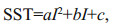 (1)
(1)where I represents SIC with a range of 0–1 (0%– 100%); a, b, and c are constant coefficients. After an improved version (2.0) of the OI analysis is developed from the OI version 1.0 (Reynolds and Smith, 1994). The OI.v2 analysis has a modest improvement in the bias correction owing to the addition of more in situ data. However, a small uncorrected residual bias of roughly -0.03℃ remains. Comparisons with other SST products show that the differences among SST products occur on space scales—and large time with monthly rms differences exceeding 0.5℃ in the Arctic where data are sparse. Because 1982 is the first year for which the data are available for the full seasons, the trend relationship between SST and SIC in 1982– 2016 is discussed below. Besides, the readers should bear in mind that the SST data used here was produced by sea ice in ice-covered areas, wherever SIC was at least 15%.
2.1.3 SAT and wind speedGridded 1.875°×1.915° daily reanalysis air temperature of 2 m level, V-wind and U-wind of 10 m level were obtained from National Center for Environmental Prediction/Department of Energy (NCEP/DOE) for the period of 1979 through 2016 (https://www.esrl.noaa.gov/psd/data/gridded/data.ncep.reanalysis2.html). The NCEP/DOE AMIP-Ⅱ Reanalysis (Reanalysis-2) based on the widely used NCEP/NCAR Reanalysis is an improved version of the NCEP Reanalysis I model that fixed errors and updated paramterizations of physical processes. The NCEP-DOE Reanalysis 2 project has incorporated upgrades to the forecast model and a diagnostic package, and is using a state-of-the-art analysis/ forecast system to perform data assimilation using past data from 1979 through the previous year. Besides, the R-1 errors in the snow cover analysis and snowmelt term had been fixed by R-2. The 2 m level SAT over water is based on a general circulation model (GCM) prediction. The inputs in the model are observed SST, observed sea ice, and atmospheric state based on a 3-D var assimilation system. The SAT over water or over sea ice is influenced by the heat flux from water or ice surface. The root-meansquare-error (RMSE) of 2 m level SAT is roughly 1.8℃ and NCEP-DOE underestimated wind speed by 1 m/s (Jakobson et al., 2012).
2.2 MethodGeographically, the Arctic consists of the Arcticbasin Ocean, adjacent seas and surrounding lands including Russia, Finland, Sweden, Norway, Iceland, Greenland (Denmark), Northern Canada and Alaska (United States). Sea ice in these different areas is subject to different climatic impacts. In order to analyze the regional variation trend of Arctic sea ice concentration, our study area is divided into nine subregions (Fig. 1) following Meier et al. (2007): the Central Arctic Ocean, Beaufort Sea, Bering Sea, Chukchi Sea, East Siberian Sea, Laptev Sea, Kara Sea, Barents Sea and Greenland Sea.

|
| Fig.1 Location map of the nine subregions used for this analysis Land is marked by white, coast by black. The sea areas or lakes outside the study area are denoted with blue. The central white circle represents the satellite observation gap by SMMR. |
Before conducting the following calculations, the grid cell sizes of the different datasets (i.e., the SST, SAT, and surface wind) are interpolated and georegistered to those of the NSIDC SIC data grids (25 km×25 km). Then the monthly trend of the SIC for a grid cell is linearly fitted over the period 1979–2016. The corresponding trends for the SAT and SW (1979– 2016) and the SST (1982–2016) are also derived. Mathematically, the retrieved linear function (y=a+bx) fits the paired data (xi, yi) by minimizing the chi-square error statistic, which is computed using Eq.2:
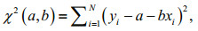 (2)
(2)where χ2 is the chi-square error statistic, i=1, 2..., N corresponds to the number of data pairs used for the fitting equation, x is the year, y is the monthly mean data for the SIC, and a and b denote the derived intercept and slope, respectively. The slope of the grid (i.e., b) represents the trend of the SIC for that grid in a specific month (January to December) over the investigated period. Bad and missing data have been removed as invalid information, and regional masks (as indicated in Fig. 1) are used to extract the information of the mean monthly SIC trends for the different subregional seas. Similarly, the corresponding trends for the other variables (the SST, SAT, and SW) are also computed. The trends are then examined using a student-test method for the confidence level. A trend analysis is also applied to retrieve the seasonal trends for the different parameters. Following the general behavior of sea ice freezing-and-melting cycles in the Arctic Ocean, we differentiate the seasons as follows: winter (January through March), spring (April through June), summer (July through September), and autumn (October through December).
To compute the correlation between any two parameters, the monthly anomaly estimates for each variable are obtained for each grid cell over the investigated period. With these anomaly estimates, the correlations for each grid cell between the SIC and the climate variables (the SAT, SST, and SW) are obtained over the investigated period. The anomaly values are computed as the difference between the monthly mean estimate and the climatology of the corresponding month for the period 1979–2010.
3 SPATIAL AND TEMPORAL VARIATIONS IN THE SIC TRENDS 3.1 Temporal variations of SIC trendsFigure 2 presents the trends and variability of SIC from 1979 through 2016 for the Arctic as a whole. Annually, there is a negative trend of -0.26±0.02%/a, reaching to a confidence level of 99%, which is consistent with earlier study (-0.28±0.03%/a) reported for November 1978 to December 1996 by Parkinson et al. (1999), and but less steep than the trend (0.31±0.04%/a) that reported by Comiso (2001) for the period of 1981 to 1999.

|
| Fig.2 Trends and seasonal and interannual variability of Arctic SIC for the years 1979–2016 The line denotes the least squares fitted through the data points, "S" represents the slope, "SIG" is the significance, "P" indicates the Pearson correlation coefficient. The winter, spring, summer, and autumn values cover the months January–March, April–June, July–September, and October–December, respectively. |
Seasonally, the highest trend is -0.43±0.03%/a in summer, followed by a weakened trend of -0.31±0.04%/a in autumn, -0.20±0.02%/a in spring, and -0.13±0.02%/a in winter. All these listed quantities are significant at a 99% level.
Figure 2 also suggests that the interannual oscillations of SIC is significant during the period of 1979 to 2016. The SIC variability in winter and spring are very similar that strenuous oscillations throughout the whole period. However, It has a different oscillations in summer, autumn, and annual average, wherein the SIC time series generally fluctuate weakly from 1979 through 1983, followed by a strong oscillations from 1984 through 1996, and steady decreased in the period of 1997 to 2006, and then followed by a violent oscillations from 2007 through 2016.
Despite of these large interannual variability, the SIC for the Arctic is showing a robust decline for the period investigated. These facts have been widely documented since the Arctic may be on the verge of a fundamental transition toward a seasonal ice cover (Stroeve et al., 2013). The rise of SST, thinning of the pack ice, making large areas prone to becoming icefree during the summer melt season, coupled with an unusual pattern of atmospheric circulation would be the key factors behind these records ice loss in recent decades (Maslanik et al., 2007a; Nghiem et al., 2007; Stroeve et al., 2013). The accelerated trends of decline seemed to be enhanced by the record lows that frequently occurred since the beginning of the 21st century. Clearly, satellite-observed record lows of Arctic sea ice extent have been reset three times, in 2007, 2012, and 2016, respectively, which corresponding to 40.56%, 39.98%, and 37.86% of the climatology value (1979–2016). The nine subregions also reveal a significant decline (99% level), except for Bering Sea and Greenland Sea (see Section 3.2 for more details) where sea ice generally vanishes in summer months.
3.2 Regional SIC trendsThe spatial distribution patterns of the SIC trends for each season are presented in Fig. 3. During the winter (Fig. 3a), a clearly decreasing SIC trend of approximately -2% per year (significant at the 99% level) is observed on the North Atlantic Ocean side (i.e., the Barents Sea, southern Greenland Sea, and southern Baffin Bay). In these areas, warmer northward-flowing Atlantic water is expected to heat the surface water and thus contribute to the significant decreases in the SIC. In contrast, a narrow belt of increased SIC values is found in the northern Bering Sea with a magnitude of -0.5%/a (not statistically significant). During the spring (Fig. 3b), the marginal seas including the Beaufort Sea (-0.20%/a), Chukchi Sea (-0.21%/a), Laptev Sea (-0.21%/a), Kara Sea (-0.51%/a), and Barents Sea (-0.75%/a) experienced a more significant reduction in their SIC trends compared to those during the winter period. However, the SIC trends in the Greenland Sea and Baffin Bay are not as strong as those during the winter. In addition, the decrease in the SIC in the northern Hudson Bay (approximately -1%/a, significant at 99%) is apparent. Meanwhile, the negative SIC trend in the Bering Sea is weaker during the spring, and it shrank to a smaller extent compared to the SIC during the winter.

|
| Fig.3 Seasonal SIC trends in the Arctic Ocean for the period 1979–2016 |
During the summer (Fig. 3c), the extensive sea ice cover in the Arctic Ocean, especially over the marginal seas (from the Beaufort Sea westward through to the Kara Sea), are observed with significantly decreased SIC trends. In these areas, the SIC trends are generally decreasing at a rate faster than -1.5%/a (significant at the 99% level). Decreased SIC trends are also identified over the channels and passages between the scattered islands in the western Canadian Archipelago. Interestingly, the Barents Sea shows a consistent and significant SIC decrease for all of the seasons except the summer. During the autumn, the areas that have significantly decreasing SIC trends retreat to smaller areal extents toward the periphery of the Arctic Ocean relative to the summer, but their distributions are still broader than those during the spring and winter seasons.
Temporal variations in the SIC ablation trends among the Arctic sub-regions are indicated in the variations of the monthly trends (Fig. 4), for which the detailed statistics are summarized in Table 1. From January to May, the variations in the monthly sea ice trends for the most parts (except the Barents Sea) are small (Fig. 4), ranging from -0.40%/a (May in the Kara Sea, significant at a 99% confidence level) to 0.07%/a (April in the Bering Sea, 90% level). The Barents Sea shows a faster SIC decrease than the other regions, ranging between -0.69% (March, 99% level) and -0.82%/a (April, 99% level). After June, the negative trends of sea ice in the Beaufort Sea, Chukchi Sea, Laptev Sea and Kara Sea become distinct and commonly reach maximum declination rates in September. Beginning in October, the SIC trends in the aforementioned marginal seas shift to a slower rate of decrease. From November to December, the decreasing SIC trends in these regions are further reduced. Among the investigated areas, the Barents Sea stands out with the smallest SIC decrease occurring during the summer rather than the winter in contrast with the other areas (Fig. 3). The SIC trends in the Laptev Sea and Greenland Sea are relatively stable, which is suggested by their overall weak seasonal variations (Fig. 4).

|
| Fig.4 Monthly trends of sea ice concentrations (%/a) in the Arctic Ocean for the different sub-regions |
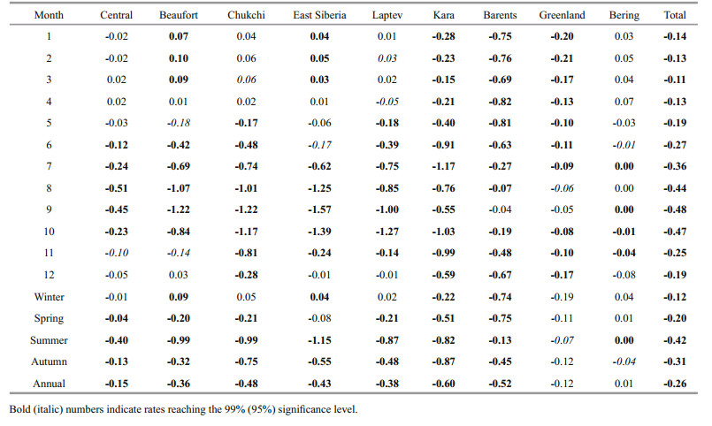
Table 1 lists the monthly, seasonal and annual SIC trends for each sub-region. Regarding the overall Arctic Ocean, the SIC trend is negative for each month and is significant at the 99% level. The maximum (minimum) SIC decreasing trend occurred in September (March) with a rate of -0.48%/a (-0.11%/a), which is significant at the 99% level. Regarding the overall Arctic Ocean sea ice, the summer and autumn experienced mean rates of -0.42%/a and -0.31%/a, respectively, which are approximately two times the rates for the winter (-0.12%/a) and spring (-0.20%/a). Annually, the SIC has a mean rate of -0.26%/a (significant at the 99% level) for the overall region, and the most rapid declines are observed for the Kara Sea (-0.60%/a) and Barents Sea (-0.52%/a), followed by the Chukchi Sea, East Siberian Sea, Laptev Sea, and Beaufort Sea (Fig. 4 and Table 1). Pack ice is common in the Central Arctic Ocean where a small declining trend in the SIC is found (-0.15%/a). The decline in SIC in the Greenland Sea is modulated by the exportation of sea ice through the Fram Strait where a larger ice outflow is likely to neutralize the regional SIC decrease due to a warmer climate. Therefore, a small SIC rate of decline is expected in the Greenland Sea (-0.12%/a, not statistically significant). Meanwhile, the Bering Sea is vulnerable to complex processes forced by oceanic and atmospheric circulations, resulting in a slightly and unnoticed positive annual trend (0.01%/a).
3.3 Linkage between SIC and interannual and decadal oscillationsWith regard to atmospheric forcing of the Arctic sea ice, many studies focused mainly on the Arctic Oscillation (AO) (Rigor et al., 2002; Holland, 2003; Zhang et al., 2003), the North Atlantic Oscillation (NAO) (Jung and Hilmer, 2001; Holland, 2003; Seierstad and Bader, 2009; Strong et al., 2009), and Dipole anomaly (DA) (Wu et al., 2006). Rigor et al. (2002) showed that international variations (from the 1980s to the 1990s) in the wintertime AO imprint a characteristic signature on SAT anomalies over the Arctic regions, and shown that the memory of the wintertime AO persists through the majority of the subsequent year: autumn and spring SAT and summertime SIC are all deeply correlated with the AO for the previous winter. Besides, they indicated that at least part of the thinning of sea ice in the Arctic Ocean recently can be ascribed to the trend in the AO toward the high-index (standard deviation > 1.0) polarity. The NAO enhanced from the 1970s to the mid-1990s, conducing to an increase of a warming North Atlantic. The increased heat convey extended throughout the North Atlantic into the Barents Sea, and finally into the Arctic Ocean, devoting to a rapid reduction of sea ice during the 1990s to the 2000s (Zeng and Delworth, 2015). Wu et al. (2006) suggested that DA mainly shown international variations from the 1980s to the 2000s. The effects of the variations include an increase in sea ice export out of the Arctic basin through the northern Barents Sea and the Fram Strait during DA positive phase, a weakening of the Beaufort gyre, and sea ice exports decrease from the Arctic basin flowing into the northern Barents Sea and the Nordic seas due to the strengthened Beaufort gyre during negative phase (standard deviation < -1.0) of DA.
Interannual variations of standardized annual AO, DA, NAO, and SIC, shown in Fig. 5, exhibit multifarious features. The time series of SIC embodying an intense decadal variations, with a distinct demarcation point 2001, can be separated into the first (1979–2001) and second (2002–2016) time periods. The first period shows positive phase, which is different from the second period. The variations of AO and NAO are similar extremely, and show pronounced decadal variations. It is mainly shown a negative phase in 1979–1994, positive phase in 1995– 2010, and turn into a positive phase during 2010–2016 for the NAO. The decadal variations of AO close to that of NAO, and the strong correlation between them is 0.76. There is a normal negative correlation (-0.43) between DA and NAO. All correlations mentioned above are with confidence levels of 95% or higher. The interaction between climate index and sea ice is not simple and concrete.

|
| Fig.5 Interannual variations of annual AO, DA and NAO index and annual SIC for 1979–2016 Lines of AO, DA, NAO, and SIC are marked by red, green, blue, and black respectively. All the data have been normalized. |
To investigate the nexus between climate indices and SIC over the ice-covered areas, regressions maps of the annual mean fields of SIC onto the AO (Fig. 6a), DA (Fig. 6b), and NAO (Fig. 6c) index were given in this paper. Features of SIC regressed on the AO is similar to corresponding features based on the NAO, but regions with mathematical statistics are different. AO drives a strong SIC negative anomaly (-15%) in the East Siberian Sea, yet NAO drives considerably a SIC positive anomaly (6%) in the Baffin Bay and Davis Strait. The SIC patterns regressed on the DA show two centers with opposite signs over the eastern and the western Arctic: one center is over eastern Laptev Sea and northern Eurasia, and the other is over Fram Strait and northern Greenland Sea, which is in accordance with the view of Wu et al. (2006) and Ikeda et al. (2001). DA drives considerably SIC negative anomaly (-6%) in the eastern Laptev Sea, and become weak gradually in all directions. Besides, the Fram Strait SIC is affected by DA significantly (7%). This may confirm that DA will promote sea ice export out of the Arctic basin into Greenland Sea, which can increase the SIC in the Fram Strait. The low correlation seemingly between the AO/NAO and the SIC (Fig. 6) reflected that sea ice provides memory for the Arctic climate system so that changes in SIC driven by the AO/NAO can be felt during the ensuing seasons. The climate indices effects appear on SIC with some phase lags offers the hope of some predictability, which may be useful for navigation along the Northern Sea route.

|
| Fig.6 Regression maps of annual SIC Regressions on the AO (a), DA (b), and NAO (c), and black lines represent significant over the 95% confidence level. |
The regional connection between SIC and SST is an issue deserving of study, although the SST values are mostly induced from the SIC values in the areas with sea ice covers higher than 15%. Figure 7 shows that the fierceness heating rate of SST is mainly in summer and autumn, but not significant in spring and winter, which is in tune with SIC trends (Fig. 3).The most drastical positive trends occured in the southern Greenland Sea (0.09 k/a, in summer), the southern Barents Sea (0.08 k/a, in autumn) and the western Bering Sea (0.07 k/a, in summer). However, the drastical decrease SIC trends took place in the northern Barents Sea (-2%/a, in winter), the central section of Beaufort Sea (-1.8%/a, in summer) and the north of the Chukchi Sea (-1.8%/a, in summer). Significantly, the major SIC trends located near latitude 75° (Fig. 3), and that of SST were occurred at the south of the latitude 70° (Fig. 7). Namely, analysis of SIC and SST based on subregions (Fig. 1) is not appropriate, particularly in the Bering Sea, Barents Sea and Greenland Sea. In this case, we calculated the average sea ice extent in winter during 1982 to 2016 (Fig. 8), and just count the trend and correlation within the ice-covered areas for winter.

|
| Fig.7 Seasonal SST trends in the Arctic Ocean for the period 1982–2016 |

|
| Fig.8 Subregions and ice-covered areas used for analysis of SIC and SST The yellow lines represent the average sea ice extent in winter over the period 1982-2016, used for limiting the statistics in the icecovered areas. |
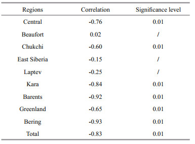
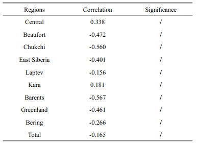
Regionally, the areas with higher correlations obtained between the winter average SST and SIC fields in the ice-covered areas for the period 1982– 2016 (Table 2) are mainly located around the marginal shelf seas, e.g., the Kara Sea (-0.84), Barents Sea (-0.92), and Bering Sea (-0.93) wherein the removal of sea ice cover contributes to a warmer surface airflow. In the Central Arctic Ocean, the two variables also correlate well (R=-0.76). The significant SIC decrease over the Central Arctic Ocean, especially for the summer and autumn, contributes to a local increase in the SST. All these correlations past the 99% significance test. According to the Fig. 9, the enervate increasing SIC trend occured in the Beaufort Sea (0.65%/dec), East Siberian Sea (0.32%/dec).On the contrary, the ice in Kara Sea and Greenland Sea retreated rapidly, and the fastest decreasing SIC trend -9.67 %/dec is in the Barents Sea, which is more than seven times the velocity of that in the whole Arctic ice-covered areas.
|

|
| Fig.9 Regional trends of SIC and SST over the ice-covered areas during the period of 1982 to 2016 Histogram marked red means no statistically significant, and without marked red represents significant over the 95%. |
A seemingly unexpected positive correlation between the SST and SIC is encountered in the northwest of the Greenland Sea, and near the eastern border of Greenland, although it is general negative correlation in the ice-covered Greenland Sea. Since the Greenland Sea is open to downstream-flowing warm seawater adjacent to the North Atlantic Sea, SST variations (0.03 k/a) are readily subject to the mixed effects of heat transport from northwardflowing oceanic flows (warming effects) and southward ice exportation (cooling effects). Net changes in the SST are thus determined by these two factors in addition to local sea ice concentration variations. Provided that more sea ice exportation and the associated melting of sea ice occurs surrounding the northern Greenland Sea, large-scale surface freshening, which could suppress oceanic mixing and lead to subsequent surface cooling, is expected (Kwok et al., 2005). Some cooling effects (-0.03 k/a) have been observed in the northern Greenland Sea (south of the Fram Strait) (Fig. 7), which is likely due to the increased sea ice areal flux through the Fram Strait (Smedsrud et al., 2017). Therefore, cooler SSTs (-0.03 k/a) together with decreasing SIC trends (-0.6%/a) jointly produce a plausible positive correlation between the variations of the two variables. In the Kara Sea, a lower negative correlation (-0.84) between the SIC and SST is likely linked to anomalous freshwater inflow from land rivers, which oppresses any immediate relationship between the SIC and SST. That the winter average SST have increase 0.14 degrees explains -6.04% of winter SIC reduction (R2=0.70) in the Kara Sea ice-covered areas during 1982–2016. The involved sea ice reduction is -50 849.25 km2. But it doesn't mean that -6.04% of SIC reduction is only caused by warmer SST. Sea ice melt is a little bit more complex and depends not just on SAT, SW and SST but on a host of heat fluxes.
The northern sector of the Barents Sea is another area wherein a reduced SIC (-1.5%/a) (Fig. 3c) in observed in concert with cooler SSTs (-0.05 k/a) (Fig. 7c), while there is an overall strong negative correlation (-0.92) between SST and SIC over the icecovered areas in the Brents Sea. According to statistical calculation, in winter, the average SST have increase 0.63 degrees explains -28.69% of SIC reduction (R2=0.85) in the Barents Sea ice-covered areas during 1982–2016, which is closely related to the sea ice ablation of 255 520.312 5 km2. Following Long and Perrie (2017), the changes in the ocean temperature in the Barents Sea is determined via the surface energy balance. They argued that reduced sea ice cover in the northern Barents Sea increases not only the amount of solar radiation absorbed by the ocean but also the quantity of heat lost at the ocean surface through turbulent heat fluxes and longwave radiation. As a result, the increased heat loss to the atmosphere due to sea ice removal likely results in a decrease in the SST. For the ice-covered Bering Sea, the close correlation between the SST and SIC is -0.93, although complex forcing from oceanic and atmospheric circulations (Wang et al., 2009). The whole Arctic sea ice-covered areas wherein a reduced SIC (-1.25%/dec) (Fig. 3c) in observed in concert with cooler SSTs (-0.02 k/dec) (Fig. 7c), while there is an overall strong negative correlation (R=-0.83) between SST and SIC over the ice-covered areas. This means that 0.07-degree growing higher of SST explains 3.02% of related SIC decrease in the winter for the period 1982–2016. Actually, the areas with SIC lower than 15%, in which SST could be really the main mechanism to control SIC.
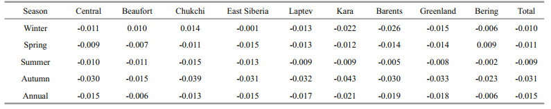
4.2 Connections with the SATDifferent from SST, the SAT trend has two peaks in one year (April and October) (Fig. 11) and affected the Arctic sea ice in various ways. Global SAT increases are mainly controlled by the radiative effects due to increased greenhouse gases. During the winter (Fig. 10a) and autumn (Fig. 10d), the warm air from the south is consistently advected toward the Barents Sea and Kara Sea, contributing to the significant melting and decreasing SIC trends (-1.5%/a) in the marginal seas of those two regions (Fig. 3a, d). Meanwhile, extensive SIC decreases (-0.48%/a in summer) in the marginal seas (Fig. 3) expose additional open water to heat the surface air, and thus, warmer SATs are expected (Fig. 10). Generally, the spatial distribution of significantly decreasing SIC trends (-0.6%/a to -2%/a in Fig. 3) is consistent with the areas that exhibit remarkable increases in the SAT (0.08 k/a to 0.3 k/a in Fig, 10), which is particularly evident for the winter (Fig. 10a vs Fig. 3a) and autumn (Fig. 10d vs Fig. 3d) seasons. By statistical analysis, a loss of 279 852.70±13 725.75 km2 of sea ice cover in the Barents Sea in response to 3.99 degrees increase of the annual SAT during 1979–2016. In the Kara Sea, a great deal of heat is carried to the ocean due to 4.84 degrees increase of the annual SAT during 38 years, reducing 190 721.45±14 728.15 km2 of sea ice cover. Besides, the annual SAT with 3.01 degrees increase is accompanied by 1 296 710.55±71 460.95 km2 of sea ice melting for the whole study area. Moreover, the geographic extent of increased SATs (clearer in Fig. 10a, d) is generally broader than that of decreased SIC trends (Fig. 3). This is likely triggered by winddriven air transport toward the inner areas of the Arctic Ocean, as illustrated by the wind vector arrows in Fig. 10.

|
| Fig.11 Trends of SAT over the Arctic Ocean for the period of 1979–2016 |

|
| Fig.10 Seasonal SAT trend over the Arctic Ocean for the period 1979–2016 Corresponding trends of surface winds (arrows) are superimposed. |
It is interesting to note that the increase in the SATs (0.03 k/a) during the summer (Fig. 10c) is less striking compared with those during the other three seasons. Figure 11 also confirms that the monthly variability in the SAT over the Arctic Ocean is large and that trends of higher SATs (up to 0.2 k/a) occurred during the winter, spring, and autumn months while weaker trends (as little as 0.06 k/a) are found during the summer. Since solar insolation rather than SIC variations predominates the variations in the SAT during the summer months, the relationship between the SIC and the SAT for the summer season appears to be less robust than for the other seasons. In addition, sea ice surface melting during the summer is favorable for the accumulation of melt ponds atop the sea ice surface. Accordingly, the distinct surface temperature difference between sea ice and open water-covered regions identified during the colder seasons reduces drastically during the summer (Comiso and Hall, 2014). Therefore, the substantial removal of sea ice cover during the summer does not effectively increase the SAT at that time.
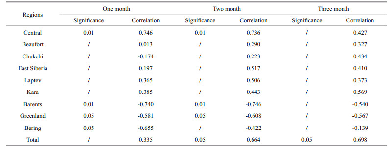
The impacts of the SAT on the SIC are variable depending on the area. In-phase correlations between the monthly fields of the SAT and SIC are generally low (-0.16) to moderate (-0.57) (Table 3). Nevertheless, a lagged correlation analysis ahead by one to three months suggests that SAT variations can explain a fraction of the SIC changes in the Central Arctic Ocean, Barents Sea, Bering Sea, and Greenland Sea (Table 4). Recent observations have revealed thinner sea ice in the Arctic Ocean sea ice cover, which can be partly attributed to warmer surface air temperatures together with a shortened freezing period during the cold seasons. Thinner ice is usually a prerequisite during the spring for the substantial sea ice loss in the following summer. Therefore, the decreases in SIC within the Arctic Ocean shelf seas during the summer (Fig. 3c) and autumn (Fig. 3d) are most vulnerable to the rising surface temperatures during autumn through to spring (Fig. 10d, a, and b).
|
|
The consecutive occurrence of record low sea ice extents (during the summer) over the past decade was partly influenced by SW forcing (Kwok, 2009; Zhang et al., 2013). Surface wind (SW) contributes to the SIC variations through thermodynamic and dynamic processes. The thermodynamic effects are most significant in the Barents-Kara Seas during the winter (Fig. 12a) and autumn (Fig. 12d) when dramatic reductions in the SIC are partly attributable to the northward transport of heat by SW.

|
| Fig.12 Seasonal trends in SW (arrows) over the period 1979–2016 Background colors denote the SIC trend (as shown in Fig. 3) for the same period. |
Dynamic impacts on sea ice retreat can be explained by two aspects. First, wind-driven sea ice can transport sea ice from the Arctic shelf seas (including the Chukchi Sea, East Siberian Sea, Laptev Sea, and Kara Sea) northward across the central ocean toward the Atlantic sector via three passages: the Fram Strait, the passage between Svalbard and Franz Josef Land (S-FJL), and that between Franz Josef Land and Severnaya Zemlya (FJL-SZ) (Rigor et al., 2002; Kwok, 2009). Furthermore, as the recent outflow of summer ice through the Fram Strait has been increasing (Bi et al., 2016; Smedsrud et al., 2017), a large-scale decline in the SIC has been observed over the Pacific sector in the Arctic Ocean (Kwok, 2008). Second, trends of the SW (0.065 m/(s·a)) during the summer (Fig. 12c) show a circulation pattern supporting the transport of sea ice cover from the Beaufort Sea westward to the southern Chukchi and East Siberian Seas (SCESS), wherein dramatic ice loss has been identified from satellite images. As more sea ice cover is removed from the SCESS, the processes governing the lateral and bottom melting of sea ice are reinforced through albedo feedback mechanisms. This could cause a further and dramatic loss of sea ice in the Arctic Ocean. For instance, the 2012 minimum sea ice extent was linked to the activity of a cyclone (Zhang et al., 2013), which occurred in August and brought a large section of ice to the SCESS, whereupon it melted away. The primary source of energy for ice melting in this case was from solar heating due to the largely reduced sea ice extent and surface albedo in the Pacific sector of the Arctic Ocean (Perovich et al., 2008).
Here, we present calculations of thermodynamic effects of climatic parameters on sea ice by sea ice growth model (Maykut et al., 1992; Parkinson et al., 1979). The bulk expressions of the sensible heat fluxes H↓ are
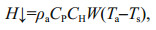 (3)
(3)where ρa is density of air (1.292 8 kg/m3), CP is the specific heat capacity of air at the near-surface level (1.004 8×10³ J/(kg·K)), CH is transfer coefficient for sensible heat (1.75×10⁻³), W is the average value of the wind speed, Ta is near-surface air temperature, Ts is skin temperature, and it's initial estimate mean values are 255 K in winter, 264 K in spring, 273 K in summer, and 259 K in autumn for the Arctic Ocean (Wang and Key, 2005a).
The ice surface net heat flux is a total of sensible heat, latent heat, solar radiation flux, long-wave flux of cloud, long-wave flux of ice, etc. But in this paper we only investigated the impact of sensible heat on sea ice and keep the sum of other energies as a constant Qt. The rate of sea ice growth can be calculated by the Eq.4. QI represents the heat of fusion of ice, set at 302 MJ/m3 (Parkinson and Washington, 1979). The thermal conductivity of the ice kI is 2.04 W/(m·k). hI is the sea ice thickness of the previous time step, and the initial estimate mean values of it are 3.9 m in winter, 4.2 m in spring, 3.2 m in summer, 3.4 m in autumn in the Arctic Ocean (Rothrock et al., 1999; Guo et al., 2010a, b, 2012, 2014). The bottom temperature of the ice is assumed to be the freezing point of seawater (271.2 K). Although Ts and hI in different subregions are distinct respectively, here we get respectively the estimate mean values of Ts and hI in the Arctic Ocean for the different seasons for the purpose of easy estimation. Actually, the mean values have modest effects on the estimate results.
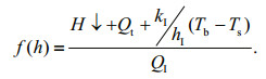 (4)
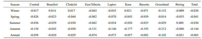
(4)The results reflected by table 5 are based on ice growth model in ice-covered areas and show that sea ice estimated decrease rates are in tune with the observed results. All subregions of the Arctic have varying degrees of ablation due to air temperature increase during the period 1979–2016, especially the Kara Sea and Barents Sea. In the Kara Sea, 0.132 degree warmer air gives 0.826 W/m2 extra sensible heat flux on sea ice, reducing 0.021 m sea ice in a year, and 0.222 degree SAT rise transfers 1.646 W/m2 extra sensible heat flux into sea ice, reducing 0.043 m sea ice growth in one autumn. Besides, the sea ice rapidest decreasing time in the entire Arctic sea icecovered areas is autumn in which 0.165 degree warmer of SAT reduces 1.351 W/m2 sensible heat into the air, retreats 0.031 m sea ice. All of these data above imply that the effects of climate parameters on sea ice are very significant. The estimate caculation of ice growth reduction due to climate parameters neglected the influences of latent heat flux, solar radiation flux, long-wave flux of cloud, long-wave flux of ice, etc. Besides, Ts and hI we used in formulas are estimates, which would lead to some errors for the result, while it can also exhibit the effects of climate parameters on sea ice to some extent. In fact, the Arctic Ocean is not covered with ice throughout the year, and there will be a large area of open water in summer. Thus, we calculated the ice growth based on the ice growth model in ice-free areas. Compared with the ice growth model in ice-covered areas (Eq.4), this formula is without thermal conductivity, and the results of the ice growth reductions are shown in Table 6. Therefore, the reasonable estimated value should be between the two extreme cases (no ice case and ice-covered case).
|
|
In order to reveal decadal variations of SIC, SAT and SW, and relationships among them, Fig. 13 was given including mean fields of SAT, SW and SIC for 1979–2001 and 2002–2016, and difference of two periods. The mean fields of those variables in first period are extremely similar to that in the second period. Compared to the first period, SAT is mainly increasing in the Eastern Hemisphere part of Arctic Ocean, in the Barents Sea particularly. The difference (b-a) between two periods is exceedingly in accordance with the trend of SAT (Fig. 13d). The difference SW (Fig. 13c) in the ice-covered areas mainly show a stronger anticyclonic Beaufort gyre that can drives the anticyclonic Beaufort gyre in sea ice motion (SIM), and further to compel sea ice enter the Transpolar Drift Stream. However, the Transpolar Drift Stream contributes to drive the sea ice export out the Arctic basin into the North Atlantic Ocean. The pattern of annual SW trends for 1979–2016 (Fig. 13d) is analogous to the difference SW between two sub periods. Similarly, the decadal variations (Fig. 13g) are mainly reflected in the marginal sea of Arctic, especially in the Northern Barents Sea, which are in line with the patterns of SIC trends for 1979– 2016 (Fig. 13h). In summary, the overall decadal variations of SAT and SW are in tune with the corresponding spatial variations of SIC.

|
| Fig.13 Mean fields, difference fields and trends of annual SAT, SW and SIC a. mean fields of annual SAT, SW (left) and SIC (right) for period of 1979-2001 (a, e) and 2002-2016 (b, f); c. represents difference (b-a), and (f) represents difference (f-e). Trends of annual SAT, SW (d) and SIC (h) for 1979-2016 at the bottom. |
The SIC trends throughout the Arctic Ocean are obtained for the period 1979–2016. Their corresponding relationships with the SST, SAT, and SW are explored. SIC trends are generally characterized by distinct seasonal and spatial variations. Seasonal decrease in the SIC are greater during the summer and autumn than those in winter and spring. Regionally, SIC reduction rates are larger over the marginal seas in the Arctic Ocean (spanning from the Beaufort Sea westward through the Barents Sea) compared with the Central Arctic Ocean, Greenland Sea, and Bering Sea. Despite of the large interannual variations, the trends of SIC for the Arctic regions are clear and basically statistically significant. These facts support that Arctic sea ice is shifting to a distinct era of decline. Sea ice provides memory for the Arctic climate system so that changes in SIC driven by the climate indices (AO, NAO and DA) can be felt during the ensuing seasons.
Strong feedbacks between the SIC and SAT are identified. Meanwhile, a lagged correlation analysis ahead by 1 to 3 months indicates the delayed impacts of the SAT on the SIC. SST variations are generally negatively correlated with variations in the SIC over the ice-covered areas. In other words, warmer sea surfaces likely cause a greater reduction in the SIC. Nevertheless, this is not always the case for the other regions. For example, decreased SSTs in the northern Barents Sea and Greenland Sea are accompanied by decreased SIC trends (i.e., they are positively correlated). The disappearance of insulating sea ice causes a cooler SST in the northern Barents Sea. With respect to the northern Greenland Sea, the increased exportation of ice via the Fram Strait and the increased ice melting therein can suppress the convective transport of heat between the underlying warm ocean and the surface water. SW can promote variations in the SIC through both dynamic (e.g., ice exportation via the Fram Strait) and thermodynamic mechanisms (e.g., the northward transport of warm and moist air over the Barents Sea). Besides, the patterns of annual SIC, SAT, SW trends for 1979–2016 are extremely analogous to the corresponding difference between the two sub periods. The overall decadal variations of SAT and SW are in tune with the corresponding spatial variations of SIC. Besides, the temperature below the surface mixed-layer may be more crucial to thermodynamics. Sea ice may melt more easily, where sea water is warmer below the surface mixed-layer. The more quantitative analyses are possible and necessary for explanation of the cause of the SIC trends (Polyakov et al., 2010). Calculation results of thermodynamic effects of climatic parameters on sea ice by sea ice growth model that sea ice estimated decrease rates are in tune with the observed results. Thus, the effects of climate parameters on sea ice are very significant.
Given the complexity of the coupled atmosphereice-ocean system in the Arctic Ocean, the influences and feedbacks of various climatic parameters on changes in the SIC require future investigation. The sea ice thickness (SIT) represents another essential parameter for quantifying the influences on sea ice due to climate changes. Compared with the SIC, the SIT represents a more integrated variable reflecting both dynamic and thermodynamic processes that act upon sea ice. Therefore, assessing variations in the SIT is a necessary subject of our future research. Fortunately, time series of satellite-derived ice thickness records have been extended to include more than a decade of data as new satellite altimeters (for example, CyroSat-2) are becoming operational. Besides, the positive ice-cloud feedback may also play a role in the ice reduction. The further work on cloud parameterization are highly requested (Ikeda et al., 2003; Wang and Key, 2005a, 5b; Liu et al., 2006, 2012; Liu and Key, 2014).
6 ACKNOWLEDGMENTThanks are given to the National Snow and Ice Data Center for providing the sea ice concentration data. The sea surface temperature (SST), air temperature, V-wind and U-wind data were obtained from the NOAA/OAR/ESRL PSD, Boulder, Colorado, USA. Thanks to Professor WU Bingyi of Fudan University for providing Dipole Anomaly (DA) data. It is thankful for the insightful comments from the two anonymous reviewers.
Bi H B, Sun K, Zhou X, et al. 2016. Arctic sea ice area export through the fram strait estimated from satellite-based data:1988-2012. IEEE Journal of Selected Topics in Applied Earth Observations and Remote Sensing, 9(7): 3144-3157.
DOI:10.1109/JSTARS.2016.2584539 |
Comiso J C, Hall D K. 2014. Climate trends in the Arctic as observed from space. Wiley Interdisciplinary Reviews:Climate Change, 5(3): 389-409.
DOI:10.1002/wcc.277 |
Comiso J C, Nishio F. 2008. Trends in the sea ice cover using enhanced and compatible AMSR-E, SSM/I, and SMMR data. Journal of Geophysical Research, 113(C2): C02S07.
|
Comiso J C, Parkinson C L, Gersten R, et al. 2008. Accelerated decline in the Arctic sea ice cover. Geophysical Research Letters, 35(1): L01703.
|
Comiso J C. 2001. Correlation and trend studies of the sea-ice cover and surface temperatures in the Arctic. Annals of Glaciology, 34: 420-428.
|
Comiso J C. 2012. Large decadal decline of the arctic multiyear ice cover. Journal of Climate, 25(4): 1176-1193.
|
Ding Q H, Schweiger A, L'Heureux M, et al. 2017. Influence of high-latitude atmospheric circulation changes on summertime Arctic sea ice. Nature Climate Change, 7(4): 289-295.
DOI:10.1038/nclimate3241 |
Francis J A, Hunter E. 2006. New insight into the disappearing arctic sea ice. Eos, Transactions American Geophysical Union, 87(46): 509-511.
|
Francis J A, Hunter E. 2007. Drivers of declining sea ice in the Arctic winter:a tale of two seas. Geophysical Research Letters, 34(17): L17503.
DOI:10.1029/2007GL030995 |
Gerdes R. 2006. Atmospheric response to changes in Arctic sea ice thickness. Geophysical Research Letters, 33(18): L18709.
|
Guo J Y, Chang X T, Cheinway H, et al. 2010a. Oceanic surface geostrophic velocities determined with satellite altimetric crossover method. Chinese Journal of Geophysics, 53(6): 2582-2589.
|
Guo J Y, Gao Y G, Chang X T, et al. 2010b. Optimal threshold algorithm of EnviSat waveform retracking over coastal sea. Chinese Journal of Geophysics, 53(2): 231-239.
DOI:10.1002/cjg2.v53.2 |
Guo J Y, Jian Q, Kong Q L, et al. 2012. On simulation of precise orbit determination of HY-2 with centimeter precision based on satellite-borne GPS technique. Applied Geophysics, 9(1): 95-107.
|
Guo J, Liu X, Chen Y, et al. 2014. Local normal height connection across sea with ship-borne gravimetry and GNSS techniques. Marine Geophysical Research, 35(2): 141-148.
DOI:10.1007/s11001-014-9216-x |
Heygster G, Alexandrov V, Dybkjær G, et al. 2012. Remote sensing of sea ice:advances during the DAMOCLES project. The Cryosphere, 6(6): 1411-1434.
DOI:10.5194/tc-6-1411-2012 |
Holl M M, Stroeve J. 2011. Changing seasonal sea ice predictor relationships in a changing Arctic climate. Geophysical Research Letters, 38(18): L18501.
|
Holland M M. 2003. The north Atlantic oscillation-arctic oscillation in the CCSM2 and its influence on arctic climate variability. Journal of Climate, 16(16): 2767-2781.
|
Holland P R. 2014. The seasonality of Antarctic sea ice trends. Geophysical Research Letters, 41(12): 4230-4237.
DOI:10.1002/2014GL060172 |
Ikeda M, Wang J, Makshtas A. 2003. Importance of clouds to the decaying trend and decadal variability in the Arctic ice cover. Journal of the Meteorological Society of Japan, 81(1): 179-189.
DOI:10.2151/jmsj.81.179 |
Ikeda M, Wang J, Zhao J P. 2001. Hypersensitive decadal oscillations in the Arctic/Subarctic climate. Geophysical Research Letters, 28(7): 1275-1278.
DOI:10.1029/2000GL011773 |
Jakobson E, Vihma T, Palo T, et al. 2012. Validation of atmospheric reanalyses over the central Arctic Ocean. Geophysical Research Letters, 39(10): L10802.
|
Jung T, Hilmer M. 2001. The link between the North Atlantic Oscillation and Arctic Sea Ice Export through fram strait. Journal of Climate, 14(19): 3932-3943.
DOI:10.1175/1520-0442(2001)014<3932:TLBTNA>2.0.CO;2 |
Kay J E, L'Ecuyer T, Gettelman A, et al. 2008. The contribution of cloud and radiation anomalies to the 2007 Arctic sea ice extent minimum. Geophysical Research Letters, 35(8): L08503.
|
Kharbouche S, Muller J P. 2017. Production of Arctic Sea-ice Albedo by fusion of MISR and MODIS data. In: Proceedings of the 19th EGU General Assembly Conference. EGU, Vienna, Austria.
|
Kwok R, Cunningham G F, Wensnahan M, et al. 2009. Thinning and volume loss of the Arctic Ocean sea ice cover:2003-2008. Journal of Geophysical Research, 114(C7): C07005.
|
Kwok R, Maslowski W, Laxon S W. 2005. On large outflows of Arctic sea ice into the Barents Sea. Geophysical Research Letters, 32(22): L22503.
|
Kwok R. 2000. Recent changes in Arctic Ocean sea ice motion associated with the North Atlantic Oscillation. Geophysical Research Letters, 27(6): 775-778.
DOI:10.1029/1999GL002382 |
Kwok R. 2008. Summer sea ice motion from the 18 GHz channel of AMSR-E and the exchange of sea ice between the Pacific and Atlantic sectors. Geophysical Research Letters, 35(3): L03504.
|
Kwok R. 2009. Outflow of Arctic Ocean sea ice into the Greenland and Barents Seas:1979-2007. Journal of Climate, 22(9): 2438-2457.
DOI:10.1175/2008JCLI2819.1 |
Laxon S W, Giles K A, Ridout A L, et al. 2013. CryoSat-2 estimates of Arctic sea ice thickness and volume. Geophysical Research Letters, 40(4): 732-737.
DOI:10.1002/grl.50193 |
Liu J P, Curry J A, Hu Y Y. 2004. Recent Arctic Sea Ice variability:connections to the Arctic oscillation and the ENSO. Geophysical Research Letters, 31(9): L09211.
|
Liu N, Lin L, Kong B, et al. 2016a. Association between Arctic autumn sea ice concentration and early winter precipitation in China. Acta Oceanologica Sinica, 35(5): 73-78.
DOI:10.1007/s13131-016-0860-7 |
Liu N, Lin L, Wang Y, et al. 2016b. Arctic autumn sea ice decline and Asian winter temperature anomaly. Acta Oceanologica Sinica, 35(7): 36-41.
DOI:10.1007/s13131-016-0911-0 |
Liu Y H, Key J R, Liu Z Y, et al. 2012. A cloudier Arctic expected with diminishing sea ice. Geophysical Research Letters, 39(5): L05705.
|
Liu Y H, Key J R, Wang X J. 2006. The influence of changes in cloud cover on recent surface temperature trends in the Arctic. Journal of Climate, 21(4): 705-715.
|
Liu Y H, Key J R, Wang X J. 2009. Influence of changes in sea ice concentration and cloud cover on recent Arctic surface temperature trends. Geophysical Research Letters, 36(20): L20710.
DOI:10.1029/2009GL040708 |
Liu Y H, Key J R. 2014. Less winter cloud aids summer 2013 Arctic sea ice return from 2012 minimum. Environmental Research Letters, 9(4): 044002.
DOI:10.1088/1748-9326/9/4/044002 |
Liu Z, Schweiger A. 2017. Synoptic conditions, clouds, and sea ice melt onset in the Beaufort and Chukchi Seasonal Ice Zone. Journal of Climate, 30(17): 6999-7016.
DOI:10.1175/JCLI-D-16-0887.1 |
Long Z X, Perrie W. 2017. Changes in ocean temperature in the Barents Sea in the twenty-first century. Journal of Climate, 30(15): 5901-5921.
DOI:10.1175/JCLI-D-16-0415.1 |
Lüpkes C, Vihma T, Birnbaum G, et al. 2008. Influence of leads in sea ice on the temperature of the atmospheric boundary layer during polar night. Geophysical Research Letters, 35(3): L03805.
|
Maslanik J A, Fowler C, Stroeve J, et al. 2007b. A younger, thinner Arctic ice cover:Increased potential for rapid, extensive sea-ice loss. Geophysical Research Letters, 34(24): L24501.
DOI:10.1029/2007GL032043 |
Maslanik J, Drobot S, Fowler C, et al. 2007a. On the Arctic climate paradox and the continuing role of atmospheric circulation in affecting sea ice conditions. Geophysical Research Letters, 34(3): L03711.
|
Maslanik J, Stroeve J, Fowler C, et al. 2011. Distribution and trends in Arctic sea ice age through spring 2011. Geophysical Research Letters, 38(13): L13502.
|
Maykut G A, Grenfell T C, Weeks W F. 1992. On estimating spatial and temporal variations in the properties of ice in the polar oceans. Journal of Marine Systems, 3(1-2): 41-72.
DOI:10.1016/0924-7963(92)90030-C |
Mei L, Xue Y, Xu H, et al. 2012. Validation and analysis of aerosol optical thickness retrieval over land. International Journal of Remote Sensing, 33(3): 781-803.
DOI:10.1080/01431161.2011.577831 |
Meier W N, Stroeve J, Fetterer F. 2007. Whither Arctic sea ice?A clear signal of decline regionally, seasonally and extending beyond the satellite record. Annals of Glaciology, 46(1): 428-434.
|
Nghiem S V, Rigor I G, Perovich D K, et al. 2007. Rapid reduction of Arctic perennial sea ice. Geophysical Research Letters, 34(19): L19504.
DOI:10.1029/2007GL031138 |
Overland J, Francis J A, Hall R, et al. 2015. The melting arctic and midlatitude weather patterns:are they connected?. Journal of Climate, 28(20): 7917-7932.
DOI:10.1175/JCLI-D-14-00822.1 |
Parkinson C L, Cavalieri D J, Gloersen P, et al. 1999. Arctic sea ice extents, areas, and trends, 1978-1996. Journal of Geophysical Research, 104(C9): 20837-20856.
DOI:10.1029/1999JC900082 |
Parkinson C L, Cavalieri D J. 2012. Arctic sea ice variability and trends, 1979-2010. The Cryosphere, 6(4): 871-880.
|
Parkinson C L, Comiso J C. 2013. On the 2012 record low Arctic sea ice cover:combined impact of preconditioning and an August storm. Geophysical Research Letters, 40(7): 1356-1361.
DOI:10.1002/grl.50349 |
Parkinson C L, Washington W M. 1979. A large-scale numerical model of sea ice. Journal of Geophysical Research, 84(C1): 311-337.
DOI:10.1029/JC084iC01p00311 |
Perovich D K, Light B, Eicken H, et al. 2007. Increasing solar heating of the Arctic Ocean and adjacent seas, 1979-2005:attribution and role in the ice-albedo feedback. Geophysical Research Letters, 34(19): L19505.
DOI:10.1029/2007GL031480 |
Perovich D K, Richter-Menge J A, Jones K F, et al. 2008. Sunlight, water, and ice:extreme Arctic sea ice melt during the summer of 2007. Geophysical Research Letters, 35(11): L11501.
DOI:10.1029/2008GL034007 |
Perovich D K, Richter-Menge J A. 2009. Loss of sea ice in the Arctic. Annual Review of Marine Science, 1: 417-441.
DOI:10.1146/annurev.marine.010908.163805 |
Polyakov I V, Timokhov L A, Alexeev V A, et al. 2010. Arctic Ocean warming contributes to reduced polar ice cap. Journal of Physical Oceanography, 40(12): 2743-2756.
DOI:10.1175/2010JPO4339.1 |
Rayner N A, Parker D E, Horton E B, et al. 2003. Global analyses of sea surface temperature, sea ice, and night marine air temperature since the late nineteenth century. Journal of Geophysical Research, 108(D14): 4 407.
DOI:10.1029/2002JD002670 |
Reynolds R W, Rayner N A, Smith T M, et al. 2002. An improved in situ and satellite SST analysis for climate. Journal of Climate, 15(13): 1609-1625.
DOI:10.1175/1520-0442(2002)015<1609:AIISAS>2.0.CO;2 |
Reynolds R W, Smith T M, Liu C Y, et al. 2007. Daily highresolution-blended analyses for sea surface temperature. Journal of Climate, 20(22): 5473-5496.
DOI:10.1175/2007JCLI1824.1 |
Reynolds R W, Smith T M. 1994. Improved global sea surface temperature analyses using optimum interpolation. Journal of Climate, 7(6): 929-948.
DOI:10.1175/1520-0442(1994)007<0929:IGSSTA>2.0.CO;2 |
Rigor I G, Wallace J M, Colony R L. 2002. Response of sea ice to the Arctic oscillation. Journal of Climate, 15(18): 2648-2663.
DOI:10.1175/1520-0442(2002)015<2648:ROSITT>2.0.CO;2 |
Rothrock D A, Yu Y, Maykut G A. 1999. Thinning of the Arctic sea-ice cover. Geophysical Research Letters, 26(23): 3469-3472.
DOI:10.1029/1999GL010863 |
Ruckert K L, Shaffer G, Pollard D, et al. 2016. The neglect of cliff instability can underestimate warming period melting in Antarctic ice sheet models. PLoS One, 12(1): e0170052.
|
Screen J A, Deser C, Sun L T. 2015. Projected changes in regional climate extremes arising from Arctic sea ice loss. Environmental Research Letters, 10(8): 084006.
DOI:10.1088/1748-9326/10/8/084006 |
Screen J A, Simmonds I. 2010. The central role of diminishing sea ice in recent Arctic temperature amplification. Nature, 464(7293): 1334-1337.
DOI:10.1038/nature09051 |
Sedlar J, Tjernström M. 2017. Clouds, warm air, and a climate cooling signal over the summer Arctic. Geophysical Research Letters, 44(2): 1095-1103.
DOI:10.1002/2016GL071959 |
Seierstad I A, Bader J. 2009. Impact of a projected future Arctic Sea Ice reduction on extratropical storminess and the NAO. Climate Dynamics, 33(7-8): 937-943.
DOI:10.1007/s00382-008-0463-x |
Serreze M C, Holland M M, Stroeve J. 2007. Perspectives on the Arctic's shrinking sea-ice cover. Science, 315(5818): 1533-1536.
DOI:10.1126/science.1139426 |
Smedsrud L H, Halvorsen M H, Stroeve J C, et al. 2017. Fram Strait sea ice export variability and September Arctic sea ice extent over the last 80 years. The Cryosphere, 11(1): 65-79.
DOI:10.5194/tc-11-65-2017 |
Stroeve J C, Serreze M C, Holland M M, et al. 2012. The Arctic's rapidly shrinking sea ice cover:a research synthesis. Climatic Change, 110(3-4): 1005-1027.
DOI:10.1007/s10584-011-0101-1 |
Stroeve J, Serreze M, Drobot S, et al. 2013. Arctic sea ice extent plummets in 2007. Eos, Transactions American Geophysical Union, 89(2): 13-14.
|
Strong C, Magnusdottir G, Stern H. 2009. Observed feedback between winter sea ice and the North Atlantic Oscillation. Journal of Climate, 22(22): 6021-6032.
DOI:10.1175/2009JCLI3100.1 |
Tschudi M A, Maslanik J A, Perovich D K. 2008. Derivation of melt pond coverage on Arctic sea ice using MODIS observations. Remote Sensing of Environment, 112(5): 2605-2614.
DOI:10.1016/j.rse.2007.12.009 |
Wang J, Ikeda M. 2000. Arctic oscillation and Arctic sea-ice oscillation. Geophysical Research Letters, 27(9): 1287-1290.
DOI:10.1029/1999GL002389 |
Wang X J, Key J R. 2005a. Arctic surface, cloud, and radiation properties based on the AVHRR polar pathfinder dataset. Part I:spatial and temporal characteristics. Journal of Climate, 18(14): 2558-2574.
|
Wang X J, Key J R. 2005b. Arctic surface, cloud, and radiation properties based on the AVHRR polar pathfinder dataset. Part Ⅱ:recent trends. Journal of Climate, 18(14): 2575-2593.
|
Wu B Y, Wang J, Walsh J E. 2006. Dipole anomaly in the winter arctic atmosphere and its association with sea ice motion. Journal of Climate, 19(2): 210-225.
DOI:10.1175/JCLI3619.1 |
Zeng F J, Delworth T L. 2015. The impact of multidecadal NAO variations on Atlantic Ocean heat transport and rapid changes in Arctic Sea Ice. In: AGU Fall Meeting.
|
EGU, Vienna Austria Zhai M, Li X, Hui F, et al. 2015. Sea-ice conditions in the Adélie Depression, Antarctica, during besetment of the icebreaker RV Xuelong. Annals of Glaciology, 56(69): 160-166.
DOI:10.3189/2015AoG69A007 |
Zhan Y Z, Davies R. 2017. September Arctic sea ice extent indicated by June reflected solar radiation. Journal of Geophysical Research, 122(4): 2194-2202.
|
Zhang J L, Lindsay R, Schweiger A, et al. 2013. The impact of an intense summer cyclone on 2012 Arctic sea ice retreat. Geophysical Research Letters, 40(4): 720-726.
DOI:10.1002/grl.50190 |
Zhang X D, Ikeda M, Walsh J E. 2003. Arctic Sea Ice and freshwater changes driven by the atmospheric leading mode in a coupled sea ice-ocean model. Journal of Climate, 16(13): 2159-2177.
DOI:10.1175/2758.1 |
Zhao J P, Cao Y, Shi J X. 2006. Core region of Arctic Oscillation and the main atmospheric events impact on the Arctic. Geophysical Research Letters, 33(22): L22708.
DOI:10.1029/2006GL027590 |