 2019, Vol. 37
Institute of Oceanology, Chinese Academy of Sciences
Article Information
- FENG Yongjiu, CHEN Lijuan, CHEN Xinjun
- The impact of spatial scale on local Moran's I clustering of annual fishing effort for Dosidicus gigas offshore Peru
- Journal of Oceanology and Limnology, 37(1): 330-343
- http://dx.doi.org/10.1007/s00343-019-7316-9
Article History
- Received Nov. 5, 2017
- accepted in principle Jan. 20, 2018
- accepted for publication Jan. 29, 2018


2 Laboratory for Marine Fisheries Science and Food Production Processes, Qingdao National Laboratory for Marine Science and Technology, Qingdao 266235, China;
3 National Distant-water Fisheries Engineering Research Center, Shanghai Ocean University, Shanghai 201306, China;
4 Key Laboratory of Sustainable Exploitation of Oceanic Fisheries Resources(Shanghai Ocean University), Ministry of Education, Shanghai 201306, China;
5 School of Earth and Environmental Sciences, the University of Queensland, Brisbane 4072, Australia;
6 Key Laboratory of Ecohydrology of Inland River Basin, Northwest Institute of Eco-Environment and Resources, Chinese Academy of Sciences, Lanzhou 730000, China
The spatiotemporal pattern of fisheries is one of the most important descriptors of offshore, and pelagic species distribution has been a source of concern in the international community for more than four decades (Rao, 1973; Gillis et al., 1993; Guidetti et al., 2003; Waluda et al., 2004; Carocci et al., 2009; Meaden et al., 2013; Feng et al., 2017a). A profound understanding of the spatiotemporal distribution of commercial fisheries is of fundamental importance to their sustainability and proper utilization (Xu et al., 2011; Feng et al., 2017b). These spatiotemporal patterns and their relationships with oceanic environmental factors can be identified using geographic information systems (GIS), spatial analysis, geostatistics, remote sensing, and related spatial technologies (Meaden and Kapetsky, 1991; Santos, 2000; Meaden, 2001; Martin, 2004; Zainuddin et al., 2004; Aswani and Lauer, 2006; Close and Hall, 2006).
Most studies of spatiotemporal patterns have been done using empirically chosen fishing grids such as 0.5°×0.5° (Chen and Chiu, 2003; Chen et al., 2003, 2007, 2008; Cao et al., 2009; Yu et al., 2016). The choice of fishing grid (also the spatial scale) substantially affects the observed spatial patterns of resources in terms of catch-per-unit-effort (CPUE), fishing effort, and catches (Tian et al., 2009, Feng et al., 2016). Using a fine 1-km spatial scale, Harford et al. (2015) simulated scenarios representing spiny lobster distribution at Glover's Reef Marine Reserve, Belize. They concluded that fishing mortality could usually be accurately estimated by mark-recovery without prior knowledge of fish transfer rates. Such fine spatial scales are not available for pelagicfi sheries. On a fine 10′ spatial scale, Saul et al. (2013) explored the spatial distribution of reef fish and estimated its spatial autocorrelation on the West Florida Shelf. Under the most widely used 30′ spatial scale, Feng et al. (2017a) explored the spatial patterns of CPUE for Ommastrephes bartramii and evaluated its variability in the northwest Pacific Ocean using the Getis-Ord Gi* statistic. Using the same 30′ scale, Yu et al. (2016) evaluated the spatiotemporal distribution and habitat hotspots of the western winter-spring cohort of O. bartramii in the northwest Pacific Ocean using CPUE and other environmental data from 1998 to 2009.
In ecological and geographical research, it has been noted that spatial patterns identified at one specific spatial scale may be valid only at this scale (Meentemeyer and Box, 1987; Turner et al., 1989; Wiens, 1989; Feng and Liu, 2015). The phenomenon has been labeled scale impact or scale effect, and has also been identified in fisheries research (Guinet et al., 2001; García-Charton et al., 2004; Tian et al., 2009; Yang et al., 2013). For example, Guinet et al. (2001) explored the spatial distribution of foraging in female Antarctic fur seals Arctocephalus gazella in relation to oceanographic variables using an integrated approach that combined a scale-dependent method and GIS. Under multiple spatial scales, García-Charton et al. (2004) investigated spatial patterns of fish assemblages and evaluated the effects of protection measures on marine reserves on western Mediterranean rocky reef fish assemblages. In a case study of O. bartramii in the northwest Pacific Ocean, Tian et al. (2009) evaluated the impact of spatial scale on fisheries and environmental data for CPUE standardization. Using multi-scale analysis, Yang et al. (2013) analyzed the distribution of CPUE and investigated the spatial variability of abundance for O. bartramii in the north Pacific Ocean; the authors suggested 30′ as a suitable spatial scale for analyzing spatial patterns of O. bartramii.
We have previously quantified the scale effects of changing spatial scales on global spatial indices and local patterns (spatial hotspots) of the squids O. bartramii and Dosidicus gigas in terms of CPUE (Feng et al., 2016, 2017a). On a global level, spatial indices studied included Moran's I Index, Geary's C, Getis-Ord General G, the average nearest neighbor and Ripley's K function. At the local level, the indices studied included mean CPUE, standard deviation (SD), skewness, kurtosis, area and centroid. We identified 25′ as the optimal scale for August and October and 20′ for September, and 50′ as the coarsest allowable spatial scale for August and October and 55′ for September. However, most studies on scale impacts were focused on CPUE while few focused on fishing effort, another important indicator of available fisheries resources (Squires, 1987; Punt et al., 2000; Bigelow et al., 2002). As a result, the impact of spatial scale on the fishing effort has yet to be fully explored, and the choice of appropriate and/or reliable scale, has yet to be made, especially at the local level.
Here, we focus on the impact of spatial scale on high values (HH) clusters identified by the Anselin Local Moran's I statistic in ArcGIS environment from D. gigas fishing effort in the waters offshore Peru. We address four questions: [1] what are the relations between the HH clusters and the spatial scales? [2] to what extent are indices of HH clusters sensitive to changes in spatial scales? [3] what are the differences of scale impacts between fishing effort and CPUE for D. gigas? and [4] what are the optimal and coarsest allowable spatial scales for spatial analysis of the fishing effort for D. gigas? The outcomes of this research may enhance our understanding of the local spatial patterns of fishing effort for D. gigas, and suggest the suitable scale of sampling for the surveying of other fishery resources.
2 MATERIAL AND METHOD 2.1 Commercial fishery dataThe jumbo flying squid D. gigas is widely distributed in the Gulf of California, the Costa Rica Dome off Central America, and the coastal and oceanic waters off Peru and Chile (Liu et al., 2013). We focus on the pelagic fisheries of Chinese fishing fleets from 2009 to 2012, using commercial fishery data provided by the Chinese Squid-jigging Technology Group (CSTG). Our study area is bounded by 78°–86°W and 8°–20°S. The raw data record the dates of fishing, fishing locations (longitude and latitude), number of fishing vessels operated per day, and the daily catch. Vessels in the Chinese squidjigging fleets were equipped with almost identical engines, lamps and fishing powers, and all operated at night (Wang and Chen, 2005). Because of these homogeneous operating characteristics (Yu et al., 2016), a standardization of the fishing effort is not required in our research. The fishing effort was calculated as:
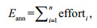 (1)
(1)where Eann is the annual fishing effort and efforti is the fishing operations for month i, within a specific fishing grid. The original data were tessellated into various fishing grids, with each fishing grid representing a square area. The length of each grid donates the grain size or spatial resolution, which substantially affects the calculation of fishing effort. The purpose of this paper is to examine the impact of grain size on the local clusters of the fishing effort.
To test the normality of fishing effort datasets, we applied Kolmogorov-Smirnov (K-S) method by taking into account their skewness and kurtosis (Zhao et al., 2014), which showed that all the raw data did not follow a normal distribution. We then conducted logarithmic transformations for 2009 and 2012, and Box-Cox transformations for 2010 and 2011, to normalize the data, making them suitable to calculate the classical statistics and linear geostatistics (Zhang et al., 2008; Cabanellas-Reboredo et al., 2011). Using normal quantile-quantile (Q-Q) plot in ArcGIS 10.1, an exploratory statistical analysis (Fu et al., 2011) has also been performed to identify the apparent outliers (extreme values), which have consequently been excluded from the calculation.
To prepare the data for multi-scale analysis, the original datasets were tessellated on twelve spatial scales from 6′ to 72′ with a scale interval of 6′ (i. e. 0.1°) between two adjacent spatial scales. Among the spatial scales, 30′ is the most widely used, not only for D. gigas but for many other pelagic species (Cao et al., 2009; Tian et al., 2009; Yu et al., 2015, 2016). The tessellation satisfies the minimum requirement of seven spatial scales for multi-scale spatial analysis (Turner et al., 1989; Wu, 2004; Feng and Liu, 2015). Some vessels recorded and reported their daily catch together with fishing locations and times, but most of the vessels reported one fishing operation for one day with the total daily catch on a very large spatial grid. As a result, the scale of original data was not included in the calculation of scale impacts for fishing effort.
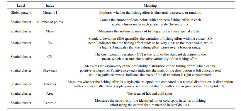
2.2 Statistics and indicesEight spatial and non-spatial statistics and indices (Table 1) were selected at global and local levels to measure the spatial distribution of fishing effort for D. gigas, and hence to investigate the scale impacts. At the global level, Moran's I statistic measures whether the pattern of fishing effort is clustered, dispersed, or random (Cliff, 1981). At the local level, the spatial clusters of fishing effort can be measured by local spatial autocorrelation statistics such as Anselin Local Moran's I (Anselin, 1995, 1996), Getis-Ord Gi* (Ord and Getis, 1995; Peeters et al., 2015), and K-means (Levine, 2015). Anselin Local Moran's I, also known as the local indicator of spatial association (LISA) (Anselin, 1995, 1996, 2004), has been widely used to identify spatial clusters and outliers in various fields (Mitchell, 2005; Zhang et al., 2008; Fu et al., 2014, 2015). Here, we used both the global and local autocorrelation statistics to examine the scale impacts on spatial clusters. Specifically, the spatial clusters at various spatial scales were identified and the change of their locations, boundaries, and statistics in response to changing spatial scale were studied in detail. Amongst the indices, the number of points, mean CPUE, SD, skewness and kurtosis are descriptive statistics, while the area and centroid are linked to boundary and location, respectively (Table 1).
|
(1) Global Moran's I
Global Moran's I is one of the most widely used global spatial autocorrelation statistics. It explores whether the pattern of fishing effort is clustered, dispersed or random based on both values and locations (Cliff, 1981). Moran's I detects the similarity of nearby fishing effort, but cannot indicate if the clustering is for high or low fishing effort. This Global Moran's I can be computed as (Sokal and Oden, 1978):
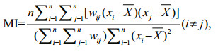 (2)
(2)where MI is the value of the Global Moran's I index; n is the number of samples of fishing effort; xi and xj are the values of fishing effort for samples i and j, respectively; X is the average value of all samples; and wij is a spatial weight matrix indicating the spatial adjacency between samples i and j, which specifies how spatial relationships among the samples are conceived. In this paper, the wij is defined using an inverse distance method (Chang, 2015), indicating that neighboring samples of fishing effort have stronger influences on a closer sample than a distant sample.
The Moran's I index ranges from -1 to 1, where MI >0 indicates clustered spatial patterns of fishing effort, MI =0 indicates a random distribution, and MI < 0 indicates dispersion. The Moran's I index is usually transformed to a z-score to determine if the observed autocorrelation is statistically significant.
(2) Anselin Local Moran's I
Anselin Local Moran's I, also known as Local Indicator of Spatial Association (LISA), measures the degree of spatial autocorrelation at each specific location (Anselin, 1995, 1996, 2004):
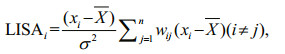 (3)
(3)where LISAi is the Local Moran's I for sample i, σ2 is the overall variance of all samples, and the n, xi, X and wij are the same as in Eq.2. The same spatial weight wij (inverse distance) as global Moran's I is used to calculate the LISA. The LISA index can be interpreted only within the context of the corresponding z-score or P-value which represents the statistical significance of the calculated statistic (Mitchell, 2005). The Cluster and Outlier Analysis tool in ArcGIS 10.1 can readily identify the clusters of fishing effort with similar values and the spatial outliers that should be excluded (Fu et al., 2014; Yuan et al., 2018). The z-score zLISAi for the statistic was calculated as:
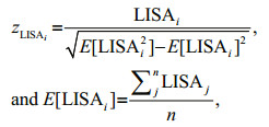 (4)
(4)where E[LISAi] represents the expectation of the local Moran's I LISAi, E[LISAi2] represents the expectation of the square of the local Moran's I LISAi, and E[LISAi]2 represents the square of the expectation E[LISAi].
A positive local Moran's I indicates that the fishing effort point is surrounded by fishing effort points with similar (high or low) values, and thus it is part of a cluster; a negative local Moran's I indicates that the fishing effort point is surrounded by dissimilar fishing effort points, and thus it is an outlier. Statistically significant clusters may consist of high fishing efforts (HH) or low fishing efforts (LL), while outliers can be a high fishing effort point surrounded by low fishing effort points (HL) or the converse, a low fishing effort point surrounded by high fishing effort points (LH). Statistically significant clusters of high fishing effort are known as hot spots; similar clusters of low fishing effort are known as cold spots.
(3) Centroids of HH clusters
Monthly fishing effort centroids were located using the Central Feature tool of ArcGIS 10.1. The centroid is the most centrally located point of the hot and cold spots for D. gigas, on differing spatial scales. The central feature, a general term in spatial statistics and distribution analysis (Khormi and Kumar, 2015), was calculated to better understand the most central point of the fishing ground and the concentration of fishing activities. The central feature is the central point in fisheries, as the features are all points. The CPUE-weighted accumulative distance from each point to every other point is considered. As a result, the point associated with the minimum accumulative distance to all other points is the centroid (Mitchell, 2005).
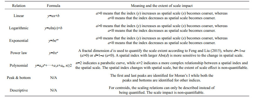
2.3 Potential scale relationsLinear, logarithmic, exponential, power law and polynomial scaling relationships have been noted in ecology (Turner et al., 1989; Wu, 2004), geography (Batty, 2005), and fisheries research (Yang et al., 2013). Here, the impacts on fishing effort were examined in consideration of each of these scaling relations (Table 2). Table 2 derived from Feng et al. (2016) shows that, y is the spatial index and x is the spatial scale. Except for the power law and polynomial relationships, a positive a indicates an increasing tendency of an index while a negative a indicates a decreasing tendency as spatial scale increases. As such, the positive or negative sign of a is a tendency indicator. Abs (a) is the absolute value of a, which is an impact indicator that suggests the extent of the scale effect.
|
For a power law relationship, negative d (with a>0) indicates that the spatial index increases as the spatial scale becomes coarser (i.e. larger fishing grid size), whereas a positive d (a < 0) indicates that the spatial index decreases as the spatial scale becomes coarser. An absolute d approaching 1 means that the spatial index is insensitive to the change of spatial scale, whereas a large absolute value d (e.g., d≥1.3) means that the spatial index is sensitive to the change of spatial scale (Feng and Liu, 2015). The extent of scale impact is not quantifiable in a polynomial scaling relationship.
3 RESULT 3.1 Impact of scale on global spatial patternsExamination of the scale impacts on global spatial patterns measured by global Moran's I benefits the investigation of spatial clusters and outliers, and helps to identify appropriate scales for spatial analysis. Figures 1a–b plot the values of Moran's I during 2009-2012. All are statistically significant, except those at 54′ to 72′ spatial scale in 2009.

|
| Fig.1 Scale impact on global spatial patterns of D. gigas offshore Peru |
The large circles in Fig. 1 indicate that Moran's I reaches peaks at the spatial scales where the clustering of spatial processes is most pronounced (Cliff, 1981; Mitchell, 2005). There are three peaks in each year during 2009-2012, and Moran's I increases from lower values at 6′ to the first peaks at 12′ in 2009-2011 and from a lower value at the original scale (1.9′) to the first peak at 6′ in 2012. This indicates that the fishing effort at the spatial scales finer those of the first peaks are more dispersed, and that the spatial patterns of fishing effort are unstable under scales finer than the first peaks. The coarsest spatial scales at which the peaks reach (i. e. the scale of the last peak) are 48′ in 2009, 2010 and 2012, and 60′ in 2011.
Figure 1c shows that z-scores of Moran's I decrease significantly as spatial scale increases in accordance with a power law relationship with R2 greater than 0.92. The fractal dimensions of the scale impacts are 2.656, 2.346, 2.06 and 2.118 for 2009-2012, successively, suggesting that the z-score of Moran's I for D. gigas is strongly sensitive to changing spatial scale. These findings are consistent with the work of Feng et al. (2016).
3.2 Scale impacts of the statistics for HH clustersThe spatial clusters and outliers of all fishing efforts were identified. For brevity, Fig. 2 only presents the spatial HH/LL clusters and outliers at four spatial scales: 10′, 30′, 60′, and 72′. Among these scales, 30′ is the most widely used. At the finest scale, all the HH/LL clusters and HL/LH outliers were identified for all years during 2009-2012. The LL clusters and outliers in 2010 and 2012 ultimately disappear at 20′, while only a few of them in 2009 and 2011 are still present as the scale becomes coarser. This indicates that, for all four years, the region that is not statistically significant become the dominant category in the study area. Consequently, the spatial patterns of fishing effort of D. gigas tend to be more homogenized with the increasing spatial scale. Therefore, instead of discussing the LL clusters and not statistically significant regions, we focus on the HH clusters because they represent the central fishing grounds.

|
| Fig.2 Clusters and outliers of D. gigas offshore Peru at 10′, 30′, 60′ and 72′ scales |
Figure 3 shows the impact of varying spatial scale on five summary statistics, including the number of points, mean effort, SD, skewness and kurtosis for the HH clusters. SD, skewness and kurtosis for 2009 cannot be computed because there is only one HH point on spatial scales from 54′ to 72′. For all four years, the number of points decreases significantly with the increase in spatial scale, showing power law scaling relations with very high R2. The fractal dimensions of the number of points are 3.234, 2.615, 2.753, and 2.726 for 2009-2012, successively, indicating that the number of points is highly sensitive to the change of the spatial scale. This scale effect is stronger than for CPUE (Feng et al., 2016).

|
| Fig.3 Scale impacts on statistics of HH clusters for D. gigas offshore Peru |
The mean fishing effort at HH clusters increases significantly with increasing spatial scale, showing a power law scale relationship with high R2. The fractal dimensions are -2.584 2, -2.696 7, -2.651 3, -2.766 6 for 2009-2012, successively. On spatial scales ranging from 6′ to 72′, mean fishing effort increases from 8 to 534 in 2009, from 8 to 595 in 2010, from 8 to 503 in 2011, and from 10 to 730 in 2012. This rapid increase is due to the accumulated fishing effort values, which are higher than the average CPUE during the tessellation. The high fractal dimensions indicate the strong scale sensitivity of HH clustering.
Similar to mean fishing effort, the SD of HH clusters follows a power law scaling relationship with negative dimensions, indicating substantial increase with the increasing spatial scale. The R2s are all larger than 0.93, and the fractal dimensions are -2.850 9, -2.477 6, -2.406 1, -2.725 8 for 2009-2012, successively. Again, the high absolute fractal dimension indicates that mean fishing effort in HH clusters is highly sensitive to changes of spatial scale. It also reveals that fishing effort for HH clusters ranges more broadly as spatial scale becomes coarser.
The CVs of the HH clusters for 2009 and 2010 follow downward quadratic polynomial relations with the changing spatial scales. The vertexes at 24′ indicate that the spatial patterns at this scale are less clustered within the HH clusters. The CV of the HH clusters for 2011 monotonically decreases with the increase of spatial scale, indicating an increasingly clustered pattern; whereas, the CV for 2012 fluctuates with the spatial scale and yields a cubic polynomial relation with low fitting performance.
For 2009 and 2012, skewness fluctuations were noted, reaching peaks at 18′ and 36′ in 2009 and at 42′ and 60′ in 2012, and reaching minimums at 12′, 30′ and 42′ in 2009 and at 36′ and 54′ in 2012 (Fig. 3d). Figure 3e shows that the scale impact on skewness follows a linear relationship in 2010 and 2011, with decreasing skewness as spatial scale increases. This also suggests that the fishing effort for HH clusters in 2010 and 2011 is increasingly asymmetrical as the spatial scale becomes coarser. Figure 3f shows that kurtosis rapidly decreases with increasing spatial scale. The scale impact displays a logarithmic relationship in 2009, 2011 and 2012, while it follows a linear relationship in 2010, suggesting that the distribution of fishing effort tends to be more platykurtic as spatial scale becomes coarser.
3.3 Scale impacts of areas for HH clustersThe areas of the D. gigas HH clusters offshore Peru are presented at spatial scales ranging from 6′ to 72′ in Fig. 4. The HH area decreases in 2009, and increases in the other three years with the increasing spatial scale. The scale impact of the HH clusters is complex; it follows a linear relationship in 2009, a convex downward quadratic relationship in 2011, and power law relationship with fractal dimensions -1.385 1 and -1.277 in 2010 and 2012, respectively. Although the number of points contained in the HH clusters decreases significantly with increasing spatial scale (Fig. 2), their area in 2010-2012 increased because of the larger fishing grid. However, the HH area in 2009 decreases because it has the highest fractal dimension (3.234) in all four years and the larger fishing grid cannot outweigh the decrease of the HH points.

|
| Fig.4 Scale impacts on HH areas for D. gigas offshore Peru |
The final index used in the characterization of the scale impact is change in location of the HH cluster centroids. Figure 5 plots the annual centroid with two-standard deviation ellipses computed using the ArcGIS 10.1 Directional Distribution tool. The cluster centroids move with changing spatial scales, but the changes are not statistically significant. Figure 5 also shows that the 2009 and 2010 ellipses are smaller than those in 2011 and 2012. This suggests that the centroids in 2009 and 2010 move over a wider range than in 2011 and 2012 along the rotation of the ellipse, which indicates the distribution direction of the centroids. Further, the HH cluster centroids in 2009 and 2012 are located to the north of the study area, but move to the south in 2010 and 2011. This indicates that the vessels moved from the north in 2009 to the south in 2010, and stayed in the south in 2011 and then moved to the north in 2012.

|
| Fig.5 The trajectories of the centroids of the HH clusters under the spatial scales from 6′ to 72′ |
We applied a multi-scale analysis to examine the scale relations of spatial clusters of the annual fishing effort for Dosidicus gigas offshore Peru. These spatial clusters were identified using local Moran's I index that may be affected by the conceptualization (weight) of spatial relationships, data transformation, and presence of extreme values. To address these issues, we used inverse distance weight, logarithmic and Box-Cox transformation, and Q-Q plot, successively. Since the focus of our paper is on scaling impacts, we do not discuss in detail how the above three factors affect the calculation of the spatial clusters. Instead, we leave the rest of valuable pages to analyze the scale relations and effects.
The scaling relations and scale effects in fisheries were grouped into six categories including linear, logarithmic, power law, quadratic polynomial, peak & bottom, and descriptive (Table 3). This means exponential scale relations that were reported in the literature (Feng et al., 2016) were not identified in the annual fishing effort data of D. gigas offshore Peru from 2009 to 2012.
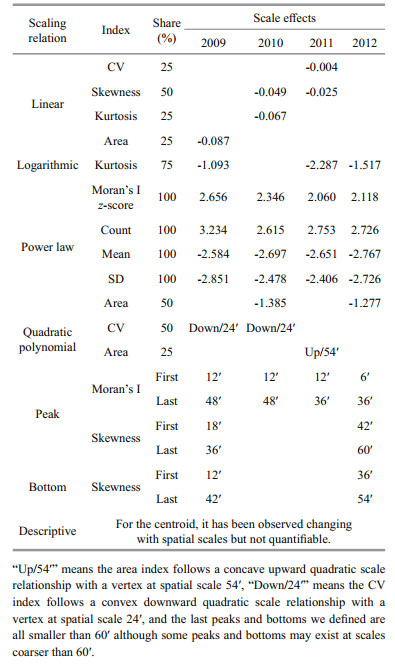
The scale effects in Table 3 show that the Moran's I z-score and the number of points contained in the HH clusters significantly decrease with the increase of spatial scale, while the mean effort and SD significantly increase with increasing spatial scale. These four indices follow power law scaling relations for all four years. The CV follows downward quadratic polynomial relations in 2009 and 2010, a negatively linear relation in 2011, and a cubic polynomial relation in 2012. The areas in 2010 and 2012 follow power law scaling relations, indicating an increasing tendency as the spatial scale become coarser; whereas, the area also follows a linear scale relation in 2009 and a quadratic polynomial scale relation in 2011.
The skewness follows a linear scale relation in 2010 and 2011 and fluctuates with spatial scale in 2009 and 2012. The kurtosis follows a logarithmic scale relation in 2009, 2011 and 2012, and a linear scale relation in 2010, indicating its decrease with the increase of spatial scale. For Moran's I, the first and last peaks were identified at the spatial scales that are finer than 60′ (Table 3). The centroids of the HH clusters are changing with spatial scales, but the extent of the scale impacts are not quantifiable.
4.2 Comparison of the scale impacts between fishing effort and CPUEWe compared the scaling impacts of fishing effort from this study with those of CPUE for O. bartramii done by Feng et al. (2018). Although mean values of fishing effort and CPUE have negative fractal dimensions, the absolute fractal dimensions of the mean effort are higher than those (< 1.5) of the CPUE in the HH clusters identified using Getis-Ord Gi*. This indicates that the mean effort is impacted more by a change in scale than the mean CPUE. For both SD and CV, the scaling relations for fishing effort are less complex than those of CPUE, because the latter follows quadratic polynomial, exponential and power law scale relations in different months.
For skewness, two scale impacts, including the peaks & bottom and the linear scale relations, were identified for fishing effort, while three scale relations including linear, quadratic polynomial and logarithmic were identified for CPUE. Except for the peaks & bottoms, all the scale relations indicate that both fishing effort and CPUE decrease as the spatial scale become coarser. For kurtosis, linear and logarithmic scale relations were identified for fishing effort while the exponential and power law scale relations were identified for CPUE. All of the scale relations of kurtosis indicate the decrease of fishing effort and CPUE with the increase of spatial scale, where the CPUE yields a stronger scale impact.
The centroid is another measure of the scale impact of fishing effort and CPUE. The centroids of the annual HH clusters of fishing effort and the monthly CPUE spatial hotspots were affected by changing spatial scale, but the effect on CPUE is much stronger.
4.3 Optimum and coarsest allowable spatial scalesAn optimum spatial scale (OP-scale) is that which best reflects the geographical features and the characteristics of fisheries resources. An inappropriate spatial scale will not accurately illustrate the generic spatial patterns of the squids, because some important information may be concealed. It has been reported that the original scale in terms of CPUE is most suitable to reflect the geographical features of the fishing data (Feng et al., 2018); however, the original data cannot sufficiently reflect the characteristics of fisheries resources because the original data are not spatially stable. The first peaks for Moran's I can be considered as the OP-scales, while the last peaks finer than 60′ can be considered as the coarsest allowable spatial scales (CA-scales).
According to the methods developed by Feng et al. (2016), the OP-scales are 12′ in 2009-2011 and 6′ in 2012, while the CA-scales are 48′ in 2009, 2010 and 2012, and 60′ in 2011, for the fishing effort of D. gigas in the waters offshore Peru (Fig. 1). Compared to CPUE, the fishing effort retrieves OP-scales that are finer, and the former reported the OP-scales at about 30′ in August and 18′ in September. The CA-scales of fishing effort are also finer than those of the CPUE, which reported the CA-scales at 54′ in August and 60′ in September.
5 CONCLUSIONWe studied the impacts of changing spatial scale on the annual HH clusters of D. gigas, as identified using Anselin Local Moran's I statistic, in the waters offshore Peru from 2009 to 2012. Our work focuses on the scaling impacts on fishing effort and considered several statistics, including the number of points, mean, SD, skewness, kurtosis, area and centroid. For a multi-scale analysis, the original fishing effort dataset of D. gigas were tessellated to twelve spatial scales from 6′ to 72′ with a scale interval of 6′. Five scaling relationships commonly used in landscape ecology and more recently in fisheries were studied: linear, exponential, logarithmic, power law, and polynomial.
Our results show that the z-score of global Moran's I and the number of points of the HH clusters follow a power law scale relationship from 2009 to 2012, showing a significant decrease with the increase of spatial scale. The mean effort and SD follow power law scaling relationships with negative dimensions from 2009 to 2012, indicating the decrease of the two indices as spatial scale become coarser. The skewness follows a linear scaling relationship for two years and fluctuates with spatial scale for the other two years, while the kurtosis follows a logarithmic scaling relationship for three years and a linear scaling relationship for another one year. In 2010 and 2012, cluster areas follow power law scaling relationship but they follow a linear scaling relationship in 2009 and a quadratic polynomial scaling relationship in 2011. Based on the peaks of Moran's I indices and the multi-scale analysis, we concluded that OP-scale is 12′ in 2009-2011 and 6′ in 2012, while the CA-scale is 48′ in 2009, 2010 and 2012, and 60′ in 2011. Our study provides a better understanding of scaling behaviors for the fishing effort of D. gigas offshore Peru and offers a method to select the best spatial scales for conducting spatial analysis of this important commercial species. We speculate that the scale impacts we identified may be applicable to other cephalopods in terms of fishing effort. Additionally, the methods presented in this paper could be applied to analyze the spatial scale effect and search for the CA-scale of other commercial species.
6 ACKNOWLEDGEMENTWe would like to thank anonymous reviewers for their helpful comments and feedback.
Anselin L. 1995. Local indicators of spatial association-LISA. Geographical Analysis, 27(2): 93-115.
|
Anselin L. 1996. The Moran scatterplot as an ESDA tool to assess local instability in spatial association. In: Fischer M M, Scholten H J, Unwin D eds. Spatial Analytical Perspectives on GIS. Taylor & Francis, London. p.111-125.
|
Anselin L. 2004. Exploring spatial data with GeoDaTM:a workbook. Center for Spatially Integrated Social Science, Urbana. 61801p.
|
Aswani S, Lauer M. 2006. Incorporating fishermen's local knowledge and behavior into geographical information systems (GIS) for designing marine protected areas in Oceania. Human Organization, 65(1): 81-102.
DOI:10.17730/humo.65.1.4y2q0vhe4l30n0uj |
Batty M. 2005. Network geography: relations, interactions, scaling and spatial processes in GIS. In: Fisher P F, Unwin D J eds. Re-presenting GIS. John Wiley & Sons, Chichester, UK. p.149-170.
|
Bigelow K A, Hampton J, Miyabe N. 2002. Application of a habitat-based model to estimate effective longline fishing effort and relative abundance of Pacific bigeye tuna(Thunnus obesus). Fisheries Oceanography, 11(3): 143-155.
DOI:10.1046/j.1365-2419.2002.00196.x |
Cabanellas-Reboredo M, Alós J, Palmer M, Grädel R, MoralesNin B. 2011. Simulating the indirect handline jigging effects on the European squid Loligo vulgaris in captivity. Fisheries Research, 110(3): 435-440.
DOI:10.1016/j.fishres.2011.05.013 |
Cao J, Chen X J, Chen Y. 2009. Influence of surface oceanographic variability on abundance of the western winter-spring cohort of neon flying squid Ommastrephes bartramii in the NW Pacific Ocean. Marine Ecology Progress Series, 381: 119-127.
DOI:10.3354/meps07969 |
Carocci F, Bianchi G, Eastwood P, Meaden G. 2009.Geographic Information Systems to Support the Ecosystem Approach to Fisheries: Status, Opportunities and Challenges. Food and Agriculture Organization of the United Nations, Rome.
|
Chang K T. 2015. Introduction to Geographic Information Systems. McGraw-Hill Education, New Delhi.
|
Chen C S, Chiu T S. 2003. Variations of life history parameters in two geographical groups of the neon flying squid, Ommastrephes bartramii, from the North Pacific. Fisheries Research, 63(3): 349-366.
DOI:10.1016/S0165-7836(03)00101-2 |
Chen X J, Chen Y, Tian S Q, Liu B L, Qian W G. 2008. An assessment of the west winter-spring cohort of neon flying squid (Ommastrephes bartramii) in the Northwest Pacific Ocean. Fisheries Research, 92(2-3): 221-230.
DOI:10.1016/j.fishres.2008.01.011 |
Chen X J, Xu L X, Tian S Q. 2003. Spatial and temporal analysis of Ommastrephe bartrami resources and its fishing ground in North Pacific Ocean. Journal of Fisheries of China, 27(4): 334-342.
(in Chinese with English abstract) |
Chen X J, Zhao X H, Chen Y. 2007. Influence of El Niño/La Niña on the western winter-spring cohort of neon flying squid (Ommastrephes bartramii) in the northwestern Pacific Ocean. ICES Journal of Marine Science, 64(6): 1 152-1 160.
|
Cliff A D. 1981. Spatial Processes: Models & Applications.Pion, London.
|
Close C H, Hall G B. 2006. A GIS-based protocol for the collection and use of local knowledge in fisheries management planning. Journal of Environmental Management, 78(4): 341-352.
DOI:10.1016/j.jenvman.2005.04.027 |
Feng Y J, Chen X J, Gao F, Liu Y. 2018. Impacts of changing scale on Getis-Ord Gi* hotspots of CPUE:a case study of the neon flying squid (Ommastrephes bartramii) in the northwest Pacific Ocean. Acta Oceanologica Sinica, 37(5): 1-10.
DOI:10.1007/s13131-018-1208-2 |
Feng Y J, Chen X J, Liu Y. 2016. The effects of changing spatial scales on spatial patterns of CPUE for Ommastrephes bartramii in the northwest Pacific Ocean. Fisheries Research, 183: 1-12.
DOI:10.1016/j.fishres.2016.05.006 |
Feng Y J, Chen X J, Liu Y. 2017a. Detection of spatial hot spots and variation for the neon flying squid Ommastrephes bartramii resources in the northwest Pacific Ocean. Journal of Oceanology and Limnology, 35(4): 921-935.
DOI:10.1007/s00343-017-6036-2 |
Feng Y J, Cui L, Chen X J, Liu Y. 2017b. A comparative study of spatially clustered distribution of jumbo flying squid(Dosidicus gigas) offshore Peru. Journal of Ocean University of China, 16(3): 490-500.
DOI:10.1007/s11802-017-3214-y |
Feng Y J, Liu Y. 2015. Fractal dimension as an indicator for quantifying the effects of changing spatial scales on landscape metrics. Ecological Indicators, 53: 18-27.
DOI:10.1016/j.ecolind.2015.01.020 |
Fu W J, Fu Z J, Ge H L, Ji B Y, Jiang P K, Li Y F, Wu J S, Zhao K L. 2015. Spatial variation of biomass carbon density in a subtropical region of southeastern China. Forests, 6(6): 1 966-1 981.
|
Fu W J, Jiang P K, Zhou G M, Zhao K L. 2014. Using Moran's I and GIS to study the spatial pattern of forest litter carbon density in a subtropical region of southeastern China. Biogeosciences, 11(8): 2 401-2 409.
DOI:10.5194/bg-11-2401-2014 |
Fu W J, Zhao K L, Zhang C S, Tunney H. 2011. Using Moran's I and geostatistics to identify spatial patterns of soil nutrients in two different long-term phosphorus-application plots. Journal of Plant Nutrition and Soil Science, 174(5): 785-798.
DOI:10.1002/jpln.v174.5 |
García-Charton J A, Pérez-Ruzafa Á, Sánchez-Jerez P, BayleSempere J T, Reñones O, Moreno D. 2004. Multi-scale spatial heterogeneity, habitat structure, and the effect of marine reserves on Western Mediterranean rocky reef fish assemblages. Marine Biology, 144(1): 161-182.
DOI:10.1007/s00227-003-1170-0 |
Gillis D M, Peterman R M, Tyler A V. 1993. Movement dynamics in a fishery:application of the ideal free distribution to spatial allocation of effort. Canadian Journal of Fisheries and Aquatic Sciences, 50(2): 323-333.
DOI:10.1139/f93-038 |
Guidetti P, Fraschetti S, Terlizzi A, Boero F. 2003. Distribution patterns of sea urchins and barrens in shallow Mediterranean rocky reefs impacted by the illegal fishery of the rock-boring mollusc Lithophaga lithophaga. Marine Biology, 143(6): 1 135-1 142.
DOI:10.1007/s00227-003-1163-z |
Guinet C, Dubroca L, Lea M A, Goldsworthy S, Cherel Y, Duhamel G, Bonadonna F, Donnay J P. 2001. Spatial distribution of foraging in female Antarctic fur seals Arctocephalus gazella in relation to oceanographic variables:a scale-dependent approach using geographic information systems. Marine Ecology Progress Series, 219: 251-264.
DOI:10.3354/meps219251 |
Harford W J, Ton C, Babcock E A. 2015. Simulated markrecovery for spatial assessment of a spiny lobster(Panulirus argus) fishery. Fisheries Research, 165: 42-53.
DOI:10.1016/j.fishres.2014.12.024 |
Khormi H M, Kumar L. 2015. Modelling Interactions Between Vector-Borne Diseases and Environment Using GIS. CRC Press, Boca Raton.
|
Levine N. 2015. CrimeStat: A Spatial Statistics Program for the Analysis of Crime Incident Locations (V 4.02). Ned Levine and Associates, Houston, Texas, and the National Institute of Justice, Washington, DC.
|
Liu B L, Chen X J, Yi Q. 2013. A comparison of fishery biology of jumbo flying squid, Dosidicus gigas outside three Exclusive Economic Zones in the Eastern Pacific Ocean. Journal of Oceanology and Limnology, 31(3): 523-533.
DOI:10.1007/s00343-013-2182-3 |
Martin K S. 2004. GIS in Marine Fisheries Science and Decision-Making. American Fisheries Society, Bethesda. p.237-258.
|
Meaden G J, Aguilar-Manjarrez J. 2013. Advances in Geographic Information Systems and Remote Sensing for Fisheries and Aquaculture. FAO, Rome.
|
Meaden G J, Kapetsky J M. 1991. Geographical information systems and remote sensing in inland fisheries and aquaculture. FAO, Rome.
|
Meaden G J. 2001. GIS in fisheries science: foundations for a new millenium. In: Nishida T, Kailola P J, Hollingworth C E eds. Proceedings of the First International Symposium on GIS in Fishery Science. Fishery GIS Research Group, Saitama, Japan. p.3-29.
|
Meentemeyer V, Box E O. 1987. Scale effects in landscape studies. In: Turner M G ed. Landscape Heterogeneity and Disturbance. Springer, New York. p.15-34.
|
Mitchell A. 2005. The Esri Guide to GIS Analysis, Volume 2:Spatial Measurements and Statistics. Esri Press, Redlands.
|
Ord J K, Getis A. 1995. Local spatial autocorrelation statistics:distributional issues and an application. Geographical Analysis, 27(4): 286-306.
|
Peeters A, Zude M, Käthner J, Ünlü M, Kanber R, Hetzroni A, Gebbers R, Ben-Gal A. 2015. Getis-Ord's hot- and coldspot statistics as a basis for multivariate spatial clustering of orchard tree data. Computers and Electronics in Agriculture, 111: 140-150.
DOI:10.1016/j.compag.2014.12.011 |
Punt A E, Walker T I, Taylor B L, Pribac F. 2000. Standardization of catch and effort data in a spatially-structured shark fishery. Fisheries Research, 45(2): 129-145.
DOI:10.1016/S0165-7836(99)00106-X |
Rao K V. 1973. Distribution pattern of the major exploited marine fishery resources of India. In: Proceedings of the Symposium on Living Resources of the Seas Around India. Mandapam Camp. http://eprints.cmfri.org.in/2688/1/Article_05.pdf
|
Santos A M P. 2000. Fisheries oceanography using satellite and airborne remote sensing methods:a review. Fisheries Research, 49(1): 1-20.
DOI:10.1016/S0165-7836(00)00201-0 |
Saul S E, Walter J E, Die D J, Naar D F, Donahue B T. 2013. Modeling the spatial distribution of commercially important reef fishes on the West Florida Shelf. Fisheries Research, 143: 12-20.
DOI:10.1016/j.fishres.2013.01.002 |
Sokal R R, Oden N L. 1978. Spatial autocorrelation in biology. 2. Some biological implications and four applications of evolutionary and ecological interest. Biological Journal of the Linnean Society, 10(2): 229-249.
DOI:10.1111/bij.1978.10.issue-2 |
Squires D. 1987. Fishing effort:its testing, specification, and internal structure in fisheries economics and management. Journal of Environmental Economics and Management, 14(3): 268-282.
|
Tian S Q, Chen Y, Chen X J, Xu L X, Dai X J. 2009. Impacts of spatial scales of fisheries and environmental data on catch per unit effort standardisation. Marine and Freshwater Research, 60(12): 1 273-1 284.
DOI:10.1071/MF09087 |
Turner M G, O'Neill R V, Gardner R H, Milne B T. 1989. Effects of changing spatial scale on the analysis of landscape pattern. Landscape Ecology, 3(3-4): 153-162.
DOI:10.1007/BF00131534 |
Waluda C M, Yamashiro C, Elvidge C D, Hobson V R, Rodhouse P G. 2004. Quantifying light-fishing for Dosidicus gigas in the eastern Pacific using satellite remote sensing. Remote Sensing of Environment, 91(2): 129-133.
DOI:10.1016/j.rse.2004.02.006 |
Wang Y G, Chen X J. 2005. The Resource and Biology of Economic Oceanic Squid in the World. Ocean Press, Beijing.
|
Wiens J A. 1989. Spatial scaling in ecology. Functional Ecology, 3(4): 385-397.
DOI:10.2307/2389612 |
Wu J G. 2004. Effects of changing scale on landscape pattern analysis:scaling relations. Landscape Ecology, 19(2): 125-138.
DOI:10.1023/B:LAND.0000021711.40074.ae |
Xu B, Chen XJ, Qian W G, Tian S Q. 2011. Spatial and temporal distribution of fishing ground for Dosidicus gigas in the offshore waters of Peru. Periodical of Ocean University of China, 41(11): 43-47.
(in Chinese with English abstract) |
Yang M X, Chen X J, Feng Y J, Guan W J. 2013. Spatial variability of small and medium scales' resource abundance of Ommastrephes bartramii in Northwest Pacific. Acta Ecologica Sinica, 33(20): 6 427-6 435.
(in Chinese with English abstract) DOI:10.5846/stxb |
Yu W, Chen X J, Chen Y, Yi Q, Zhang Y. 2015. Effects of environmental variations on the abundance of western winter-spring cohort of neon flying squid (Ommastrephes bartramii) in the Northwest Pacific Ocean. Acta Oceanologica Sinica, 34(8): 43-51.
DOI:10.1007/s13131-015-0707-7 |
Yu W, Chen X J, Yi Q, Chen Y. 2016. Spatio-temporal distributions and habitat hotspots of the winter-spring cohort of neon flying squid Ommastrephes bartramii in relation to oceanographic conditions in the Northwest Pacific Ocean. Fisheries Research, 175: 103-115.
DOI:10.1016/j.fishres.2015.11.026 |
Yuan Y M, Cave M, Zhang C S. 2018. Using Local Moran's I to identify contamination hotspots of rare earth elements in urban soils of London. Applied Geochemistry, 88: 167-178.
DOI:10.1016/j.apgeochem.2017.07.011 |
Zainuddin M, Saitoh S I, Saitoh K. 2004. Detection of potential fishing ground for albacore tuna using synoptic measurements of ocean color and thermal remote sensing in the northwestern North Pacific. Geophysical Research Letters, 31(20): L20311.
DOI:10.1029/2004GL021000 |
Zhang C S, Luo L, Xu W L, Ledwith V. 2008. Use of local Moran's I and GIS to identify pollution hotspots of Pb in urban soils of Galway, Ireland. Science of the Total Environment, 398(1-3): 212-221.
DOI:10.1016/j.scitotenv.2008.03.011 |
Zhao K L, Fu W J, Liu X M, Huang D L, Zhang C S, Ye Z Q, Xu J M. 2014. Spatial variations of concentrations of copper and its speciation in the soil-rice system in Wenling of southeastern China. Environmental Science and Pollution Research, 21(11): 7 165-7 176.
DOI:10.1007/s11356-014-2638-9 |