 2019, Vol. 37
Institute of Oceanology, Chinese Academy of Sciences
Article Information
- ZHANG Zhixiang, LIU Lingling, WANG Fan
- Oceanic barrier layer variation induced by tropical cyclones in the Northwest Pacific
- Journal of Oceanology and Limnology, 37(2): 375-384
- http://dx.doi.org/10.1007/s00343-019-8008-1
Article History
- Received Jan. 9, 2018
- accepted in principle Mar. 2, 2018
- accepted for publication May. 21, 2018


2 University of Chinese Academy of Sciences, Beijing 100049, China;
3 Qingdao National Laboratory for Marine Science and Technology, Qingdao 266071, China;
4 Center for Ocean Mega-Science, Chinese Academy of Sciences, Qingdao 266071, China
Tropical cyclone (TC) is one of extreme air-sea interaction phenomena. The powerful wind forcing of TCs can input intense energy which can generate upwelling, near-inertial waves and currents to the ocean (Price et al., 1994; Jaimes and Shay, 2009; Chang et al., 2012, 2013). The sea surface cooling is one of the obvious situations under TCs, with relatively lower temperature on the right side of TCs' track in the Northern Hemisphere (Price, 1981; Shay et al., 1992; Chu et al., 1999, 2000; Jacob et al., 2000; Zheng et al., 2008; Chiang et al., 2011; Nam et al., 2012). The upper ocean cooling is because of the entrainment of subsurface cold water (Price, 1981; Sanford et al., 1987; Bender et al., 1993; Huang and Xiao, 2009). On the other hand, it hinders TCs absorbing heat energy from the underlying ocean, which can restrain cyclones' intensification (Schade and Emanuel, 1999; Cione and Uhlhorn, 2003; Kaplan and DeMaria, 2003; Shay and Uhlhorn, 2008). Except wind forcing, the rainfall under TCs can also affect temperature and salinity in the upper ocean (Chu and Wang, 2003; Jourdain et al., 2013).
The oceanic mixed layer (ML), with quasi-uniform properties including temperature, salinity and density, is the interface of air-sea interaction. If a prominent salinity stratification emerges in a deep isothermal layer (IL) of a high freshwater input area, the density ML will be shallower than IL. The middle layer between the base of ML and IL is defined as the barrier layer (BL) (Sprintall and Tomczak, 1992; Chu and Wang, 2003). Under TCs, BL acts as a "barrier" for the entrainment and vertical mixing, and this weakens sea surface cooling, which in turn constrains the feedback of upper ocean to TCs (Wang et al., 2011; Balaguru et al., 2012; Jourdain et al., 2013; Vissa et al., 2013; Neetu et al., 2014; Androulidakis et al., 2016). Recent study suggests BL is only favorable for TCs' intensification when TC-induced forcing is strong enough to penetrate into it. The presence of BL intensifies cyclones, but the destroyed BL makes the subsequent ones weaker due to the upper ocean cooling (Androulidakis et al., 2016). Overall, BL is an important ocean layer impeding TC intensification.
Nevertheless, BL variation under TCs has not been systematically explored and researched so far. Based on Argo profiles, Fu et al. (2014) conclude the barrier layer thickness (BLT) is increased within 6 hours after strong and slow TCs' passage. With the number of Argo profiles increasing, it is appropriate to investigate the response of upper ocean to TCs. This makes thoroughly analyzing BL variation possible.
In this paper, we study BL variation induced by TCs in the Northwest Pacific, and its mechanism. The data and numerical model used in this study are described in Section 2. Section 3 depicts the BL variation induced by TCs based on Argo floats. Finally, some summaries and conclusion are presented in Section 4.
2 DATA AND METHOD 2.1 Barrier layer thicknessThe Argo profiles in the Northwest Pacific during 2000–2013, from China Argo Real-time Data Center, are used to quantify BL variation during TCs' passage. Based on Argo profiles, BLT is computed as the difference between isothermal layer depth (ILD) and mixed layer depth (MLD) (Lukas and Lindstrom, 1991; Sprintall and Tomczak, 1992). ILD is defined as the depth that temperature is 0.5℃ lower than that of reference level. MLD is defined at the depth with density difference of Δσt from the reference level, and Δσt=0.5∂σ/∂T (Sprintall and Tomczak, 1992). Since the Argo observation data of water with depth less than 10 m is scarce, 10 m depth is utilized as the reference level, which can also avoid the ocean diurnal variation (Grodsky et al., 2008; Wang et al., 2011). In addition, barrier layer depth (BLD) is the intermediate depth of BL.
2.2 TC best-track dataThe TC best track data in the Northwest Pacific, including the South China Sea, are provided by the US Navy Joint Typhoon Warning Center (JTWC) for the period of 2000–2013. Six-hour records of the position of TCs' center, the intensity, and other important parameters of TCs are included in the besttrack data, typically at 0000, 0600, 1200, and 1800 UTC.
2.3 The PWP modelThe Price-Weller-Pinkel (PWP) vertical mixing model (Price et al., 1986) is adopted to simulate the thermodynamical response of upper ocean, with the focus on BL, during moving TCs. The model accepts a series of external forcing induced by TCs, including surface heat flux, wind stress, and precipitation which are applied to the initial vertical profiles of temperature and salinity. The vertical mixing in the model mainly counts on three stability criteria (Price et al., 1986): 1) static instability; 2) mixed layer instability; 3) shear instability. The critical bulk and gradient Richardson numbers are set to 0.65 and 0.25 separately.
According to the protocols of Willoughby et al. (2006) and Rappin et al. (2013), the wind speed associated with TCs is obtained by the tangential wind speed based on the wind profile model. Wind stress is calculated using the bulk formula (Oey et al., 2006):
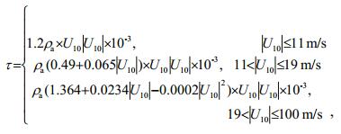
where U is the local wind speed, ρa is the density of air. This formula is modified from Large and Pond (1981) to incorporate the limited drag coefficient for high wind speeds (Powell et al., 2003).
The precipitation data is from Tropical Rainfall Measuring Mission (TRMM 3B42), with temporal resolution of 3-hour and horizontal resolution of 0.25°×0.25° (Huffman et al., 2007). Daily heat flux and evaporation data are from OAFlux with a spatial resolution of 1°×1° (Yu and Weller, 2007; Yu et al., 2008).
3 RESULT 3.1 BL variation induced by TCs based on Argo profilesThe Argo profiles are paired to analyze BL variation before and after TCs. The Argo pairs are sorted by the following criteria: (1) Both of the Argo profiles must be within the radius of 500 km to TCs' track; (2) the distance between paired profiles must be less than 50 km to minimize the difference due to background spatial ocean variability; (3) for the temporal window, the time interval of pre- and post-TCs' profiles must be restricted to 11 days; (4) for the float identity, the profile pairs must be from the same float to avoid duplicate usage of profiles and float-to-float calibration diversity. Despite above sampling criteria, numerous Argo profile pairs are satisfied that shown in Fig. 1.

|
| Fig.1 Selected Argo pairs in the Northwest Pacific during 2000–2013 The blue (red) dots represent the locations of Argo before (after) TCs' passage. |
There are two characteristic types of vertical temperature, salinity and density profiles during TCs' passage (Figs. 2 and 3). Before typhoon TEMBIN, 35 m BL exists below a vertical salinity and density gradient in the layer of 0–20 m. However, the temperature, salinity and density in the upper ocean is quasi-uniform after TEMBIN. This means TEMBIN makes the BL structure disappear at (19.94°N, 120.16°E). Another circumstance is that BL structure emerges after typhoon's passage (Fig. 3). It is apparently shown that the values of temperature, salinity and density are constant at (10.59°N, 132.51°E) in the layer of 0–70 m. Hence, no BL structure occurs before typhoon PARMA (dotted). Nevertheless, a sharp vertical salinity gradient comes into view in the layer 0–20 m after the PARMA. Collectively, TCs can evoke diametrically opposing variation of BL under various forcing. It is noticeable that BL variation is an infrequent phenomenon during TCs. Statistically, only 29% of Argo pairs shows that BLT variation is more than 5 m between pre- and post-TCs. Among this, the possibility of BL getting thicker is ca. 48%. The following discussions are on the basis of Argo pairs with BLT variation more than 5 m.

|
| Fig.2 The track of typhoon TEMBIN in 2012 and position of Argo float 5902167 (a); the temperature (red), salinity (blue) and density (black) profiles before (dotted) and after (solid) TEMBIN (b) |

|
| Fig.3 The track of typhoon PARMA in 2009 and position of Argo float 5901524 (a); the temperature (red), salinity (blue) and density (black) profiles before (dotted) and after (solid) PARMA (b) |
The spatial-temporal distributions of azimuthally averaged ILD, MLD and BLT variation (Fig. 4)., in which x-axis indicates the distance between the given Argo station and TCs' track, and y-axis implies the time after TCs' passage. The patterns of MLD and ILD are not exactly same, which will induce the variation of BL. The deepening positions of IL and ML are evidently rightward bias, with the maximal one occurring at 100–150 km right of the TCs' track, which is in accordance with previous studies (Fu et al., 2014). Furthermore, BL is mainly weakened within 7 days on the right side of TCs' passage, with the maximum value of BLT decrease emerging around 3 days after TCs. BL intensification prefers to occur far away from the left side of TCs.

|
| Fig.4 Time-space plots of the azimuthally averaged sample number (a), ILD variation (b), MLD variation (c) and BLT variation (d) with the box of 1 day × 50 km |
With BL existing before TCs, data shows that predominant TC-induced BL weakening is on the north of 20°N, where more than 60% BL structure will be destroyed by TCs. Moreover, the maximal BL weakening location appears around 30°N. On the other hand, TCs can effectively intensify BL on the south of 20°N without BL structure before TCs. However, only about 20% of samples can form a new BL structure through TCs on the north of 20°N in the Northwest Pacific (Fig. 5d). In summary, foremost TCs' weakening effects on BL are on the north of 20°N; while the intensifying impacts are centered on the south of 20°N in the Northwest Pacific.

|
| Fig.5 Numbers of Argo pairs (a), the probability of BL weakening after TCs (%) (c) and the spatial distribution of TCinduced BL variation (e) for the cases with BL existing before TCs; numbers of Argo pairs (b), the probability of BL intensification (d) and the spatial distribution of TC-induced BL variation (f) for the cases without BL before TCs The spatial resolution is 2.5×2.5°. |
The observation data of Argo float could reveal the BL variation by TCs. However, all associated physical processes (i.e. wind, precipitation, air-sea heat flux and initial ocean state) are included. It is difficult to separate out the effect of single factor on BL variation. Therefore, to further understand the effects of TCs on oceanic BL structure, the PWP model is utilized to analyze the dominant processes.
3.2.1 Model settingA typical ocean thermohaline structure with 30 m MLD and 19 m BLT is set as initial state (Fig. 6a). Wind stress, precipitation and air-sea heat flux are external forcing acting on the initial profiles. Their time evolution are obtained from the position around 50 km right away from TCs' center. Wind forcing (Fig. 6b) is achieved through the wind profile model (Willoughby et al., 2006; Rappin et al., 2013). Green, blue and red lines represent forcing under TCs with 2 m/s, 5 m/s and 8 m/s translation speed, respectively (Fig. 6b, c, d). The time variation of precipitation is acquired through TRMM 3B42 data average (Fig. 6c), with the same total amount (300 mm) under three kinds of TCs. Figure 6d demonstrates that air-sea heat flux calculated from OAFlux has symmetric variation tendency during TCs' process. Except abovementioned, the seawater-rain temperature difference is also a significant factor, however, this needs to be investigated further in the absence of observation data.

|
| Fig.6 Initial temperature (red), salinity (blue), and density (black) profiles used in the PWP model (a); wind speed (b), precipitation (c) and heat flux (d) used in model running are all from slow (green), moderate (blue) and fast (red) TCs, respectively |
Generally, the essence of BL variation is the change of temperature-salinity stratification in IL. The intensification (erosion) of BL structure is directly associated with the vertical salinity gradient enhancing (weakening) in the shallow layer. This means BL can be affected by the processes that changes the vertical stratification especially salinity profiles of the upper ocean. TCs can make above effects through vertical mixing, entrainment, precipitation and upwelling. Horizontal advection is also an influence factor, but we do not discuss it thoroughly because of the limitation of one-dimensional model.
Powerful wind stress of TCs offers enormous mechanical energy to sustain turbulent mixing process in the upper ocean. This makes properties (temperature, salinity and density) to become uniform state and it is difficult for the existence of BL in this situation. The black lines in Fig. 7 indicate the time evolution of MLD, ILD and BLT only with the wind forcing. The base of ML gradually gets deeper owing to the wind forcing, which causes BL weakening even vanishing.

|
| Fig.7 Time evolution results of MLD (a), ILD (b) and BLT (c) from one-dimensional PWP model under five kinds of external force hypothesis: wind (black), precipitation with strong wind (blue), precipitation with weak wind (green), precipitation (yellow) and heat flux (red) |
Freshwater input is an important mechanism of BL existing in ocean. Hence, precipitation accompanying TCs is a crucial factor for the BL variation. However, precipitation only spreads over the top of seawater and cannot affect the BL structure without wind mixing. The yellow lines in Fig. 7 demonstrate that the ML, IL and BL would always keep stable if there is no mixing working. Overall, wind mixing is a necessary element contributing to the freshwater penetrating into the subsurface ocean.
The combined impacts of mixing and precipitation are indicated by the blue and green lines in Fig. 7. At the beginning, the freshwater gradually permeates into the ocean, and this makes the MLD get thinner. With time going, increasing wind forcing causes the upper ocean to be homogenous If wind stress is not enough strong to reach the initial ML's base, MLD will be thinner due to the freshwater input, and BL will intensify (green line) under this situation. In brief, only precipitation cannot affect the salinity profile, but it is able to adjust the salinity and induce the BL variation with mixing. Therefore, whether BL will be intensified or not depends on the competition between wind mixing and precipitation.
Surface heat flux contributes to 15%–30% of sea surface cooling during TCs' process (Price, 1981; Vincent et al., 2012). Nevertheless, it only causes ocean temperature disturbance temporally, and the upper ocean will gradually revert back to pre-TCs' state consuming 5–20 days. It cannot induce irreversible changes for the barrier layer structure. The results of numerical experiment (red line in Fig. 7) also prove surface heat flux has no considerable impact on the BL variation.
Upwelling is an adiabatic process which can cause any entire layer moving upward. Although it cannot change the temperature-salinity stratification, BL will be affected by it if upwelling is strong enough to make the ML outcrop to air-sea interaction surface after TCs. Otherwise, upwelling could change nothing except BLD. One-dimensional model does not contain upwelling process; therefore, we cannot predict its influence through this model. Above all, local wind stress and precipitation are the predominant factors on regulating BL variation and we will conduct experiments to quantify their impacts under TCs on next step.
To examine the impacts of different factors on the BL variation, another four experiments are implemented (Table 1). Only one independent variable changes with time in each experiment, while the others remain constant. The local maximum wind speed is the independent variable in Exp.1, which primarily depends on the TCs' intensity, size and the distance from TCs' center. Exps.2, 3 and 4 are set to examine the effects of local precipitation, initial MLD and BLT, respectively. The MLD, ILD and BLT keep constant after 140 hours (Fig. 7). Therefore, the BLT variation at 144th hour in the numerical model is defined as the final state after TCs in our study.
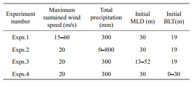
Slow TCs have more significant impacts on the ocean BLT than fast TCs, as the results of Exps.1–4 exhibited in Fig. 8. Oceanic BLT weakens more greatly under higher wind speeds, and even disappears when wind speed reaches a critical value—55 m/s under slow TCs (Fig. 8a). Fig. 8b depicts BLT variation after TCs' passage with total precipitation varying from 0 to 800 mm among them. Huge precipitation is more conducive to the presence of BL structure under moderate and fast TCs. When total rainfall exceeds 500 mm, BL will start to thicken under fast TCs. During slow TCs, due to its longer lasting time, mixing has influence on deeper levels, which is harmful for the existence of BL structure. Figure 8c shows that the BLT variation in different initial MLD states after TCs' passage. The shallower initial MLD leads to BLT reducing more, because stronger mixing near sea surface is less likely to affect BL under the deeper ML. Furthermore, if the initial BL structure does not exist, the precipitation and mixing processes will generate a new one (Fig. 8d).

|
| Fig.8 BLT variation after TCs' passage under various local maximal wind speed (a), total precipitation (b), initial MLD (c) and initial BLT (d), respectively Green, blue and red lines represent results of slow, moderate and fast TCs. |
The BLT variation during TCs' passage is investigated according to the comparisons of Argo profiles pre- and post-TCs' and one-dimensional PWP model. TCs affect BL through two approaches: 1) Enhance pre-existed BL, or even generate an entirely new BL structure; 2) weaken the original BL, or make it vanish. In the Northwest Pacific, BL attenuation is predominant near the centers of TCs, which is in accordance with Jourdain et al. (2013). The effects of TCs on the weakening of BL is principal on the north of 20°N in the Northwest Pacific. BL tends to get thicker in areas south of 20°N after TCs relatively.
Wind stress and precipitation are two dominant factors for the BL variation. Without precipitation, the effect of mixing is primarily reflected in the deepening of MLD, which goes against the maintenance of BL. The freshwater from TCs' rainfall is able to produce new salinity gradients in the upper layer, which is beneficial for generating BL structure. However, in the absence of wind-driven mixing process, it is impossible for precipitation to affect the BL structure below ML.
The strengthening or weakening of BL mainly depends on wind mixing or precipitation prevailing. The results of one-dimensional PWP model indicate that TC-induced BLT variation is linked to the local maximal wind speed, TCs' translation speed, total rainfall, initial MLD and initial BLT. If wind-driven mixing intensity is strong enough to overwhelm the effect of rainfall, the BL structure will weaken or even disappear. On the other hand, heavy rainfall also makes BL to get thicker (Fu et al., 2014) or produces a completely new one. What needs to be emphasized is that the role of wind has obvious impacts for slow TCs.
Our result is only preliminary study to explore the TC-induced BL variation. Several problems still need to be solved. For instance, there are no horizontal advection and upwelling processes in the onedimension PWP model. Besides, the effect of TCs on the upper ocean is an extremely complicated process. Some vague physical processes of TCs may lead to errors in final analysis. Consequently, the impact of TCs on oceanic BL structure remains to be investigated further.
Androulidakis Y, Kourafalou V, Halliwell G, Le Hénaff M, Kang H, Mehari M, Atlas R. 2016. Hurricane interaction with the upper ocean in the Amazon-Orinoco plume region. Ocean Dynamics, 66(1-2): 1 559-1 588.
|
Balaguru K, Chang P, Saravanan R, Leung L R, Xu Z, Li M K, Hsieh J S. 2012. Ocean barrier layers' effect on tropical cyclone intensification. Proceedings of the National Academy of Sciences of the United States of America, 109(36): 14 343-14 347.
DOI:10.1073/pnas.1201364109 |
Bender M A, Ross R J, Tuleya R E, Kurihara Y. 1993. Improvements in tropical cyclone track and intensity forecasts using the GFDL initialization system. Monthly Weather Review, 121(7): 2 046-2 061.
DOI:10.1175/1520-0493(1993)121<2046:IITCTA>2.0.CO;2 |
Chang Y C, Chen G Y, Tseng R S, Centurioni L R, Chu P C. 2012. Observed near-surface currents under high wind speeds. Journal of Geophysical Research:Oceans, 117(C11): C11026.
|
Chang Y C, Chen G Y, Tseng R S, Centurioni L R, Chu P C. 2013. Observed near-surface flows under all tropical cyclone intensity levels using drifters in the northwestern Pacific. Journal of Geophysical Research:Oceans, 118(5): 2 367-2 377.
DOI:10.1002/jgrc.20187 |
Chiang T L, Wu C R, Oey L Y. 2011. Typhoon Kai-Tak:an ocean's perfect storm. Journal of Physical Oceanography, 41(1): 221-233.
|
Chu P C, Lu S H, Liu W T. 1999. Uncertainty of South China Sea prediction using NSCAT and National Centers for Environmental Prediction winds during tropical storm Ernie, 1996. Journal of Geophysical Research:Oceans, 104(C5): 11 273-11 289.
DOI:10.1029/1998JC900046 |
Chu P C, Veneziano J M, Fan C W, Carron M J, Liu W T. 2000. Response of the South China Sea to tropical cyclone Ernie 1996. Journal of Geophysical Research:Oceans, 105(C6): 13 991-14 009.
DOI:10.1029/2000JC900035 |
Chu P C, Wang G H. 2003. Seasonal variability of thermohaline front in the central South China Sea. Journal of Oceanography, 59(1): 65-78.
DOI:10.1023/A:1022868407012 |
Cione J J, Uhlhorn E W. 2003. Sea surface temperature variability in hurricanes:implications with respect to intensity change. Monthly Weather Review, 131(8): 1 783-1 796.
DOI:10.1175//2562.1 |
Fu H L, Wang X D, Chu P C, Zhang X F, Han G J, Li W. 2014. Tropical cyclone footprint in the ocean mixed layer observed by Argo in the Northwest Pacific. Journal of Geophysical Research:Oceans, 119(11): 8 078-8 092.
DOI:10.1002/2014JC010316 |
Grodsky S A, Carton J A, Liu H L. 2008. Comparison of bulk sea surface and mixed layer temperatures. Journal of Geophysical Research:Oceans, 113(C10): C10026.
DOI:10.1029/2008jc004871 |
Huang W R, Xiao H. 2009. Numerical modeling of dynamic wave force acting on Escambia Bay Bridge deck during Hurricane Ivan. Journal of Waterway, Port, Coastal, and Ocean Engineering, 135(4): 164-175.
|
Huffman G J, Adler R F, Curtis S, Bolvin D T, Nelkin E J. 2007. Global rainfall analyses at monthly and 3-h time scales. In: Levizzani V, Bauer P, Turk F J eds. Measuring Precipitation from Space. Springer, Dordrecht, Netherlands. p.291-305.
|
Jacob S D, Shay L K, Mariano A J, Black P G. 2000. The 3D oceanic mixed layer response to Hurricane Gilbert. Journal of Physical Oceanography, 30(6): 1 407-1 429.
DOI:10.1175/1520-0485(2000)030<1407:TOMLRT>2.0.CO;2 |
Jaimes B, Shay L K. 2009. Mixed layer cooling in mesoscale oceanic eddies during hurricanes Katrina and Rita. Monthly Weather Review, 137(12): 4 188-4 207.
DOI:10.1175/2009MWR2849.1 |
Jourdain N C, Lengaigne M, Vialard J, Madec G, Menkes C E, Vincent E M, Jullien S, Barnier B. 2013. Observationbased estimates of surface cooling inhibition by heavy rainfall under tropical cyclones. Journal of Physical Oceanography, 43(1): 205-221.
|
Kaplan J, DeMaria M. 2003. Large-scale characteristics of rapidly intensifying tropical cyclones in the North Atlantic basin. Weather and Forecasting, 18(6): 1 093-1 108.
DOI:10.1175/1520-0434(2003)018<1093:LCORIT>2.0.CO;2 |
Large W G, Pond S. 1981. Open ocean momentum flux measurements in moderate to strong winds. Journal of Physical Oceanography, 11(3): 324-336.
|
Lukas R, Lindstrom E. 1991. The mixed layer of the western equatorial Pacific Ocean. Journal of Geophysical Research:Oceans, 96(S01): 3 343-3 357.
DOI:10.1029/90JC01951 |
Nam S, Kim D J, Moon W M. 2012. Observed impact of mesoscale circulation on oceanic response to Typhoon Man-Yi (2007). Ocean Dynamics, 62(1): 1-12.
|
Neetu S, Lengaigne M, Vincent E M, Vialard J, Madec G, Samson G, Ramesh Kumar M R, Durand F. 2014. Influence of upper-ocean stratification on tropical cyclone-induced surface cooling in the Bay of Bengal. Journal of Geophysical Research:Oceans, 117(C12): C12020.
|
Oey L Y, Ezer T, Wang D P, Fan S J, Yin X Q. 2006. Loop current warming by hurricane Wilma. Geophysical Research Letters, 33(8): L08613.
DOI:10.1029/2006gl025873 |
Powell M D, Vickery P J, Reinhold T A. 2003. Reduced drag coefficient for high wind speeds in tropical cyclones. Nature, 422(6929): 279-283.
DOI:10.1038/nature01481 |
Price J F, Sanford T B, Forristall G Z. 1994. Forced stage response to a moving hurricane. Journal of Physical Oceanography, 24(2): 233-260.
|
Price J F, Weller R A, Pinkel R. 1986. Diurnal cycling:observations and models of the upper ocean response to diurnal heating, cooling, and wind mixing. Journal of Geophysical Research:Oceans, 91(C7): 8 411-8 427.
DOI:10.1029/JC091iC07p08411 |
Price J F. 1981. Upper ocean response to a hurricane. Journal of Physical Oceanography, 11(2): 153-175.
|
Rappin E D, Nolan D S, Majumdar S J. 2013. A highly configurable vortex initialization method for tropical cyclones. Monthly Weather Review, 141(10): 3 556-3 675.
DOI:10.1175/MWR-D-12-00266.1 |
Sanford T B, Black P G, Haustein J R, Feeney J W, Forristall G Z, Price J F. 1987. Ocean response to a hurricane. Part I:observations. Journal of Physical Oceanography, 17(11): 2 065-2 083.
|
Schade L R, Emanuel K A. 1999. The ocean's effect on the intensity of tropical cyclones:results from a simple coupled atmosphere-ocean model. Journal of the Atmospheric Sciences, 56(4): 642-651.
DOI:10.1175/1520-0469(1999)056<0642:TOSEOT>2.0.CO;2 |
Shay L K, Black P G, Mariano A J, Hawkins J D, Elsberry R L. 1992. Upper ocean response to Hurricane Gilbert. Journal of Geophysical Research:Oceans, 97(C12): 20 227-20 248.
DOI:10.1029/92JC01586 |
Shay L K, Uhlhorn E W. 2008. Loop current response to hurricanes Isidore and Lili. Monthly Weather Review, 136(9): 3 248-3 274.
DOI:10.1175/2007mwr2169.1 |
Sprintall J, Tomczak M. 1992. Evidence of the barrier layer in the surface layer of the tropics. Journal of Geophysical Research:Oceans, 97(C5): 7 305-7 316.
DOI:10.1029/92JC00407 |
Vincent E M, Lengaigne M, Madec G, Vialard J, Samson G, Jourdain N C, Menkes C E, Jullien S. 2012. Processes setting the characteristics of sea surface cooling induced by tropical cyclones. Journal of Geophysical Research:Oceans, 117(C2): C02020.
|
Vissa N K, Satyanarayana A N V, Kumar B P. 2013. Response of upper ocean and impact of barrier layer on Sidr cyclone induced sea surface cooling. Ocean Science Journal, 48(3): 279-288.
DOI:10.1007/s12601-013-0026-x |
Wang X D, Han G J, Qi Y Q, Li W. 2011. Impact of barrier layer on typhoon-induced sea surface cooling. Dynamics of Atmospheres and Oceans, 52(3): 367-385.
DOI:10.1016/j.dynatmoce.2011.05.002 |
Willoughby H E, Darling R W R, Rahn M E. 2006. Parametric representation of the primary hurricane vortex. Part Ⅱ:a new family of sectionally continuous profiles.. Monthly Weather Review, 134(4): 1 102-1 120.
DOI:10.1175/MWR3106.1 |
Yu L S, Jin X Z, Weller R A. 2008. Multidecade global flux datasets from the objectively analyzed air-sea fluxes(OAFlux) project: latent and sensible heat fluxes, ocean evaporation, and related surface meteorological variables.Woods Hole Oceanographic Institution, Woods Hole, Massachusetts. p.64.
|
Yu L S, Weller R A. 2007. Objectively analyzed air-sea heat fluxes for the global ice-free oceans (1981-2005). Bulletin of the American Meteorological Society, 88(4): 527-540.
DOI:10.1175/BAMS-88-4-527 |
Zheng Z W, Ho C R, Kuo N J. 2008. Importance of pre-existing oceanic conditions to upper ocean response induced by Super Typhoon Hai-Tang. Geophysical Research Letters, 35(20): L20603.
DOI:10.1029/2008GL035524 |