 2019, Vol. 37
Institute of Oceanology, Chinese Academy of Sciences
Article Information
- GAO Jiaxiang, ZHANG Rong-Hua, WANG Hongna
- Mesoscale SST perturbation-induced impacts on climatological precipitation in the Kuroshio-Oyashio extension region, as revealed by the WRF simulations
- Journal of Oceanology and Limnology, 37(2): 385-397
- http://dx.doi.org/10.1007/s00343-019-8065-5
Article History
- Received Mar. 27, 2018
- accepted in principle Apr. 24, 2018
- accepted for publication May. 2, 2018


2 University of Chinese Academy of Sciences, Beijing 100049, China;
3 Laboratory for Ocean Dynamics and Climate, Qingdao National Laboratory for Marine Science and Technology, Qingdao 266237, China
In the last decades, satellite observations have discovered ubiquitous mesoscale (horizontal scales of 10-100 km) features in the ocean and atmosphere all over the world (Chelton et al., 2004; Chelton and Xie, 2010). In the ocean, persistent mesoscale sea surface temperature (SST) perturbations are found to be associated with oceanic frontal zones, mesoscale eddy activities and the tropical instability waves (TIW). It is widely recognized that at large scales the extratropical ocean is forced by the atmosphere (Xie, 2004). At mesoscale, however, low-level wind speed perturbations are highly correlated with SST perturbations, implying the ocean is forcing the atmosphere (Chelton and Xie, 2010). Due to its important implications for regional climate and weather prediction, a lot of research efforts have been devoted to understanding this mesoscale air-sea interaction utilizing theories (Lindzen and Nigam, 1987; Hayes et al., 1989; Wallace et al., 1989), observations (Small et al., 2008; O'Neill et al., 2010b, 2012), and numerical models (Bryan et al., 2010; O'Neill et al., 2010a; Zhang, 2014).
The Kuroshio is one of the two strongest western boundary currents in the Northern Hemisphere. The confluence of the Kuroshio and the southwardflowing Oyashio and their eastward extensions create the Kuroshio-Oyashio Extension (KOE) region. This region features abundant mesoscale SST perturbations associated with the oceanic fronts, meanders of the extension currents and mesoscale eddies. The linear relationship between the perturbations of SST and near-surface winds in this region, which is referred to as the mesoscale SST-wind coupling, has been identified by both satellite observations (Nonaka and Xie, 2003; O'Neill et al., 2010a, 2012) and model simulations (Bryan et al., 2010; Putrasahan et al., 2013) and agrees well with the linear relation derived from other regions of the world (Small et al., 2008; Bryan et al., 2010; O'Neill et al., 2010b). In addition, it has long been noted that the mesoscale SST features in the KOE region, especially the related oceanic SST fronts, are able to exert an influence on the large-scale mean atmospheric circulation and climate. Based on observational evidence and reanalysis data, Nakamura et al. (2004) suggested there exists a close association between the mid-latitude storm track and oceanic fronts. Taguchi et al. (2009) found that oceanic SST fronts in the KOE region act to enhance the meridional gradients of the turbulent heat and moisture fluxes and facilitate the storm-track development. Tokinaga et al. (2009) pointed out that the Kuroshio Extension front plays an important role in modifying local cloud-top height as well as sea fog frequency and may help maintain the baiu rainband east of Japan. Using regional atmospheric simulations, Iizuka (2010) demonstrated that when fine-scale SST is prescribed as the SST boundary conditions in the KOE region, interannual precipitation variation is enhanced in areas downwind of the mesoscale SST perturbations. Ma et al. (2015), using both satellite observations and numerical simulations, indicated that active Kuroshio eddy activities result in more winter precipitation along the Kuroshio and less precipitation along the northwest coast of the U.S. Recently, Ma et al. (2016) and Wei et al. (2017) found that mesoscale air-sea interaction also affects the mean state of the Kuroshio Extension.
Although studies mentioned above have made significant progress in understanding the effects of mesoscale SST perturbations, the link between the low-level atmospheric responses and the related climatological impacts have not been fully understood because the former is thought to be confined to the boundary layer (Taguchi et al., 2009). Based on 5-year operational analysis data and atmospheric general circulation model (AGCM) simulations, Minobe et al. (2008) pointed out that a persistent rain band is anchored along the Gulf Stream by local boundary layer responses to the enhanced SST gradient in the frontal zone, suggesting a pathway by which the nearsurface atmospheric responses can extend beyond the boundary layer and influence regional climate. It remains an important question whether a similar rectified effect of mesoscale SST perturbations can be identified in the KOE region and explained by the same mechanism because the environmental conditions in this region are unique and different from those in the Gulf Stream.
The purposes of the present study are thus to examine the climatological precipitation response to the mesoscale SST perturbations in the KOE region and explore the underlying mechanisms using the Weather Research and Forecasting (WRF) Model with high-resolution regional atmospheric simulations during 10-year periods. Two simulations are performed, in which one is forced by low-resolution SST and another by additional high-resolution mesoscale SST perturbations extracted from satellite observations. Comparisons are made between these two simulations to isolate the mesoscale SST effects on the atmosphere, with a focus on precipitation. The rest of this paper is organized as follows. In Section 2, we describe the regional atmospheric model, the experimental setup and data used in this study. In Section 3, after validating the model results, we demonstrate the climatological precipitation response to the mesoscale SST perturbations and examine the mechanisms. The discussions are given in Section 4, followed by conclusions in Section 5.
2 DATA AND METHODIn this study, we adopted the WRF Model V3.8.1 to simulate the atmospheric responses. The WRF model is a state-of-the-art community atmospheric model developed for both atmospheric research and operational weather forecasting application. The WRF model in this study uses the Advanced Research WRF (ARW) dynamic core (Skamarock et al., 2008).
The WRF model provides a flexible sets of physics options including various parameterization schemes. Perlin et al. (2014) showed that the planetary boundary layer (PBL) scheme is crucial for an accurate representation of the mesoscale SST-wind coupling, which is fundamental to the atmospheric responses of interest in this study. So we chose the GrenierBretherton-McCaa (GBM) PBL scheme (Bretherton et al., 2004), which has been reported to reproduce the boundary layer responses that are best consistent with the Quick Scatterometer (QuikSCAT) observations among the eight schemes investigated (Perlin et al., 2014). In addition, we chose the Lin et al.'s scheme (1983) for microphysics, the Kain-Fritsch scheme (Kain, 2004) for cumulus parameterization and the revised Fifth-Generation Penn State/NCAR Mesoscale Model (MM5) surface layer scheme (Jiménez et al., 2012).
The model domain covers the Northwest Pacific from 25°N to 50°N and 130°E to 180°E with the KOE region located almost at the center. The horizontal resolutions in both directions are 25 km using a Lambert projection. In the vertical, the model consists of 31 levels. The time step is 90 s. The simulation period is from September 1, 2004 to March 1, 2014 and the results are output at daily intervals. For the atmospheric initial and boundary conditions, we adopted the National Centers for Environmental Prediction (NCEP) FNL (Final) Operational Model Global Tropospheric Analyses data (ds083.2). The FNL data are available at 6-h intervals on a 1°×1° grid. The atmospheric boundary conditions are also updated at 6-h intervals.
The experimental methodology followed from Zhang et al. (2014) for studying the TIW-induced SST forcing effects. In this work, we performed two simulations that differed only in the prescribing of monthly varying SST boundary conditions for the WRF model. The SST boundary conditions for the control run (CTRL) were derived from the NCEP FNL SST data available at 6-h intervals on a 1°×1° grid. The FNL SST was averaged to obtain monthly fields, which were then interpolated into model grids. Mesoscale oceanic features are almost absent from the FNL SST due to its low spatial resolution. For the perturbation run (PER), the WRF model was additionally forced by mesoscale SST perturbations derived from the optimally-interpolated (OI) SST product version 4.0. That is, the derived SST perturbations were also interpolated into model grids and then added onto the FNL SST used in CTRL on a monthly basis. The OI SST is created from the microwave (MW) and infrared (IR) satellite observations and available at daily intervals on a 9 km×9 km grid at the Remote Sensing Systems. To extract the SST perturbations, a 2D LOESS (locally weighted smoothing) smoother (Schlax and Chelton, 1992; Schlax et al., 2001) was used with a 15° (longitude)×5° (latitude) cut-off wavelength. First, the low-pass-filtered SST was obtained by applying the LOESS smoother to the monthly-averaged OI SST. Then the smoothed SST was subtracted from the original fields to extract mesoscale SST perturbations for each month, a procedure similar to Wei et al. (2017). This experimental setup allows us to directly attribute the differences between the two simulations to the mesoscale SST perturbations we added.
Satellite observations of ocean surface wind and precipitation were used to validate the model results. For the near-surface wind, we used the daily u and v components of the 10-m wind speed from Version-4 data products of the QuikSCAT available at the Remote Sensing Systems in 0.25° spatial resolution. For precipitation, we used the Tropical Rainfall Measuring Mission (TRMM) Multi-satellite Precipitation Analysis (TMPA) 3B43 monthly precipitation averages which are also available in 0.25° spatial resolution. The TMPA 3B43 data were downloaded from the Asia-Pacific Data-Research Center (APDRC) Live Access Server (LAS) 7.
3 RESULT 3.1 Simulated mesoscale SST-wind couplingBefore examining the precipitation simulated by WRF, it is necessary to validate our experimental setup. Minobe et al. (2008) suggested that the lowlevel wind response is responsible for inducing local rainfall changes. Ma et al. (2015) found a cohesive response to the mesoscale SST perturbations in the boundary layer height and convective precipitation. These results indicate the low-level atmospheric responses can extend beyond the boundary layer and influence precipitation. So it is important to make sure that the WRF model in this study is able to reproduce the low-level atmospheric responses, which are characterized by a positive correlation between the perturbations of SST and near-surface winds, with a reasonable strength and spatial pattern.
Figure 1 shows the 10-m wind speed perturbations derived from QuikSCAT and WRF along with the SST perturbations extracted from the OI SST in January 2009 in the KOE region. This boreal winter month was randomly chosen for an easier comparison with previous studies (O'Neill et al., 2010b; Putrasahan et al., 2013) which have pointed out that the mesoscale air-sea interaction is the strongest and most evident in winter. To obtain the 10-m wind speed perturbations from QuikSCAT data, a high-passfiltering process similar to what we did to the OI SST was applied to the monthly scalar-averaged 10-m wind speed field using a 2D LOESS smoother with a 20° (longitude)×10° (latitude) cut-off wavelength. For the model results, we first calculated the monthly scalar-averaged 10-m wind speed from daily output for CTRL and PER, respectively, then the wind speed perturbations were calculated as PER minus CTRL. The use of daily QuikSCAT observations makes sure the result is comparable with that derived from WRF. In Fig. 1a, the mesoscale SST field is mainly characterized by randomly distributed cold and warm perturbations. The positive correlation between the perturbations of 10-m wind speed and SST is indicated by increased (decreased) wind speed over warm (cold) SST perturbations. This spatial pattern of 10-m wind response is well captured by the WRF model as demonstrated by Fig. 1b even though both wind field perturbations exhibit some kind of noise. The 10-m wind speed perturbations reproduced by the WRF model also show a good consistency with previous results obtained by Bryan et al. (2010) and Putrasahan et al. (2013) using different models.

|
| Fig.1 The 10-m wind speed perturbations (m/s) for (a) QuikSCAT and (b) WRF simulations in contours, with colors indicating SST perturbations (℃) from the OI SST in January 2009 The contour intervals are 0.2 m/s, with solid (dashed) lines representing positive (negative) values, and the zero contour being omitted for clarity. |
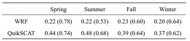
To make a quantitative and more robust evaluation of the WRF simulations, we calculated statistics of the linear relation between the mesoscale perturbations of monthly mean 10-m wind speed and SST from 34°N to 42°N, and 144°E to 164°E. This sub-region features the strongest mesoscale SST perturbations in the KOE region. The wind speed perturbations were linearly regressed on the SST perturbations and the slope of the regression line was defined as the mesoscale SSTwind coupling strength. The coupling strengths for each season (spring: March to May; summer: June to August; fall: September to November; winter: December to February) were calculated using monthly WRF output from 2005 to 2013 as well as monthly QuikSCAT data from 2005 to 2008. These monthly fields were averaged from daily data. The results are presented in Table 1 along with corresponding correlation coefficients. It is evident that the WRF model in this study reproduces a weaker SST-wind coupling strength than that derived from QuikSCAT observations. Similar discrepancies have been previous reported by Song et al. (2009) and Bryan et al. (2010) using different models. They suggested that the weaker coupling strength results from the limitations of the boundary layer parameterization in the atmospheric models because the SST-wind coupling strength is highly dependent on boundary layer processes. Table 1 also indicates that the coupling strength between the mesoscale perturbations of 10-m wind speed and SST in our WRF simulations shows little seasonal variation and thus is unaffected by the amplitude of the mesoscale SST perturbations, which is weakest in summer and strongest in winter. This is consistent with Perlin et al. (2014) and suggestive of the primary role of linear processes.
|
Although the simulated 10-m wind speed response is weaker, the correlation coefficients for all the linear regressions we have calculated are greater than 0.5, indicating a good positive correlation between the perturbations of 10-m wind speed and SST in our WRF simulations. The spatial pattern of simulated 10-m wind perturbations is also in good agreement with QuikSCAT observations and previous modeling studies. These indicate our experimental setup is able to capture the boundary layer responses to the mesoscale SST perturbations in the KOE region well, allowing us to explore their effects on climatological precipitation.
3.2 Precipitation response in the KOE region 3.2.1 Climatological precipitationIn Fig. 2, we present the climatological precipitation (mm/d) in the KOE region averaged from 2005 to 2013 for the TMPA 3B43 data and the two WRF simulations. The original TMPA data are available in mm/h, so they were multiplied by 24. It can be easily noted that in the KOE region, the climatological precipitation simulated by the WRF model in both CTRL and PER is higher than the TMPA result. This discrepancy is actually not surprising because it has been pointed out that the TRMM precipitation radar algorithm tends to underestimate precipitation outside the tropics (Huffman et al., 2017). So we instead pay more attention to the comparison of the spatial distributions of climatological precipitation between WRF and TMPA. Figure 2a shows that in the KOE region, the observed climatological precipitation features a broad northeast-southwest-oriented rain band. Maximum climatological precipitation in this region is located offshore from approximately 140°E to 150°E. Its position generally corresponds to the Kuroshio Extension, implying an anchoring effect of the warm SST. Both CTRL and PER successfully reproduce this spatial pattern of the climatological precipitation as indicated by Fig. 2b, c. A major discrepancy between CTRL and PER is revealed by a closer examination on the fine-scale structures of the climatological precipitation. Magnitude of the gradient of the climatological precipitation in the dashed rectangular areas in Fig. 2 is showed in Fig. 3. In the TMPA data (Fig. 3a), a band of enhanced gradient extending from 35°N to the northeast can be observed. This feature can be clearly identified in Fig. 3c (PER) but is missed in Fig. 3b (CTRL), which indicates that the WRF model produces a more realistic spatial distribution of the climatological precipitation in PER. So the mesoscale SST perturbations are important for an accurate representation of climatological precipitation in the KOE region. Local features can be lost if lowresolution SST is prescribed as SST boundary conditions to force the atmospheric models even though the horizontal resolutions of the atmospheric model are high enough to simulate these features.

|
| Fig.2 Climatological precipitation (mm/d) averaged in 2005–2013 for (a) TMPA 3B43, (b) CTRL and (c) PER The dashed rectangles indicate the location of enhanced gradient. |

|
| Fig.3 Magnitude of the gradient of the climatological precipitation (mm/d per 100 km) in the dashed rectangular areas in Fig. 2 for (a) TMPA 3B43, (b) CTRL and (c) PER |
To examine the details of the climatological precipitation response to the mesoscale SST perturbations, difference in the climatological precipitation between CTRL and PER (PER minus CTRL) is demonstrated in Fig. 4a along with the mean mesoscale SST averaged over the same time period, i.e., from 2005 to 2013. Near the east coast of Japan (see the leftmost red dashed rectangular area in Fig. 4a), the SST perturbations are characterized by positive perturbations on one side and negative perturbations on another, indicating a strong oceanic SST front exists in this area. This SST front forms due to the contrast between the warm Kuroshio and cold nearshore water as the Kuroshio separates from the coast, so it is almost a permanent feature in the mesoscale SST perturbations and cannot be removed by time-averaging. Hereafter this front is referred to as the Kuroshio front.

|
| Fig.4 Differences between CTRL and PER (PER minus CTRL) in climatological fields calculated in 2005–2013 a. total precipitation; b. convective precipitation; c. non-convective precipitation (mm/d); d. 10-m wind convergence (10-6/s); e. vertical velocity at 800 hPa (10-3 m/s); f. sea level pressure laplacian (10-8 Pa/m2). The overlaid contours indicate mean OI SST perturbations (℃) averaged in 2005-2013. The contour intervals are 0.2℃, with solid (dashed) lines representing positive (negative) values, and the zero contour being omitted for clarity. The red dashed rectangles indicate the three oceanic frontal zones. |
In Fig. 4a, two more oceanic SST fronts are revealed by the mean mesoscale SST field. One is located near 40°N, 150°E (the middle red dashed rectangular area in Fig. 4a) and another is located near 42°N, 167°E (the rightmost red dashed rectangular area in Fig. 4a). These two fronts have been demonstrated to be closely associated with dynamics of the Oyashio Extension (OE) by previous studies (Isoguchi et al., 2006; Qiu et al., 2017). In the rest of this paper they are referred to as the west-OE front and east-OE front respectively as in Qiu et al. (2017). Above results show that unlike a single continuous front in the Gulf Stream, the KOE region comprises three quasipermanent separate oceanic SST fronts owing to its unique current dynamics.
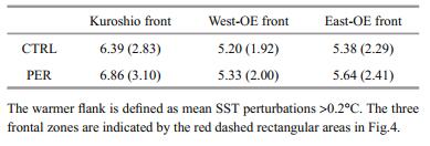
3.2.3 Precipitation response to the SST frontsEvident precipitation response can be identified in Fig. 4a near the east coast of Japan and corresponds well with the Kuroshio front. Climatological precipitation increases (decreases) on the warmer (colder) flank of the Kuroshio front, resulting in locally enhanced precipitation gradient mentioned above. Similar climatological precipitation response can also be observed in the west-OE front and the east-OE front. Table 2 shows the statistics of the climatological precipitation and the standard deviation of monthly mean precipitation rate over the warmer flank (defined as mean SST perturbations > 0.2℃) of the three SST frontal zones, respectively. It is indicated that the climatological precipitation increases from 6.39 mm/d to 6.86 mm/d on the warmer flank of the Kuroshio front, which is about 7.4% of enhancement. For the west-OE and east-OE front, the enhancement is 2.5% and 4.8%, respectively. In addition, positive SST perturbations in the three frontal zones enhance local precipitation variability as evident by higher standard deviation. We also calculate the mean precipitation response over the whole frontal zones (not shown), and the results suggest the net effect of the SST fronts is to increase local precipitation, which is consistent with the rectified effect of mesoscale SST perturbations described by Ma et al. (2015).
|
The precipitation enhancement along the fronts in the KOE region resembles the rain band found by Minobe et al. (2008) and Kuwano-Yoshida et al. (2010) along the Gulf Stream SST front, but the extent and amplitude of our simulated precipitation response are not comparable with theirs because they used a different smoothing method with a longer cut-off wavelength. However, the relatively short cut-off wavelength of the 2D LOESS smoother helps us reveal the fine-scale structure of the oceanic SST fronts in the KOE region and gain a better understanding of how these fronts affect the climatological precipitation. In this region, each of the three SST fronts is able to exert a rectified effect on local precipitation and the climatological precipitation response is characterized mainly by the sum of independent responses to each front.
3.2.4 Mechanism for the precipitation responseIn Fig. 4b, c, we separate the difference in climatological precipitation between CTRL and PER further into the convective part and non-convective part to assess their relative contributions. It is worth noting that this result is based on the model output so it is sensitive to the choices of the microphysics scheme and cumulus parameterization in the WRF model, but it can still help us gain more insight into how additional precipitation is produced by WRF in response to SST perturbations. In Fig. 4b, the convective precipitation response corresponds well with the three SST fronts. The non-convective precipitation difference in Fig. 4c shows no clear spatial pattern so it is hard to infer there is a direct link between the non-convective precipitation response and the mesoscale SST perturbations. These results suggest that the climatological precipitation response to the SST fronts in this region is dominated by changes in convective precipitation. This is consistent with the result presented by Kuwano-Yoshida et al. (2010). They analyzed the precipitation response to the Gulf Stream front and found the convective precipitation is most strongly affected by the locally enhanced SST gradient.
The dominant role of convective precipitation response can be explained by the mechanism proposed by Minobe et al. (2008). They suggested that locally enhanced SST gradient in the frontal zone induces near-surface wind convergence on the warmer flank of the front through the pressure adjustment mechanism. Low-level convergence causes local upward motion that can reach the free atmosphere. This facilitates the supply of moisture and heat to a higher level over the warmer flank, leading to more frequent deep convection. So more convective precipitation occurs along the Gulf Stream and a climatological rain band can be observed.
Since Minobe et al. (2008) focused only on the rain band along the Gulf Stream, it remains to be examined whether the same mechanism is also at work in the KOE region. In Fig. 4d, e, f, the differences in three climatological fields between CTRL and PER (PER minus CTRL) are presented. These climatological fields are derived by averaging the monthly meanfi elds from 2005 to 2013. Figure 4d shows that compared with CTRL, enhanced 10-m wind convergence can be observed in PER on the warmer flank of all three SST fronts and the divergence is also enhanced on the colder flank. In Fig. 4e, the difference in vertical velocity at 800 hPa corresponds well with the low-level convergence in Fig. 4d. A similar response in vertical velocity can still be discernable at 500 hPa (not shown), suggesting the upward motion induced by the low-level convergence can reach the free atmosphere. A correspondence between the difference in sea level pressure laplacian in Fig. 4f and 10-m wind convergence indicates the pressure adjustment in the boundary layer causes low-level wind response to the fronts as suggested by Minobe et al. (2008). These results indicate a remarkable consistency between the climatological precipitation response to the SST fronts in the KOE region and the anchoring of a rain band by the Gulf Stream front. Although in our experiment the SST fronts in the KOE region are relatively weak in strength and discontinuous in space, they still exert an important rectified effect on regional climatological precipitation through the pressure adjustment to the enhanced SST gradient.
3.2.5 Seasonal variation in the precipitation responseFigure 5 shows the differences in daily precipitation histograms between CTRL and PER for each season over the three frontal zones. The histograms are derived from daily precipitation data from 2005 to 2013 using all grid points in the respective dashed rectangular areas. Generally, the differences are most pronounced in winter. The frequency of 0 to 10 mm daily precipitation is decreased while the frequency of 10 to 40 mm daily precipitation is increased. This is consistent with Ma et al. (2015), who found increased frequency of heavy rain events along the Kuroshio when mesoscale SST perturbations are not smoothed out in their WRF simulations. For the Kuroshio front (the leftmost column), similar increases in heavy rain events can also be identified in other three seasons but the precipitation responses are relatively weak in spring and summer (Fig. 5b, c). For the west-OE front (the middle column) and the eastOE front (the rightmost column), although in winter (Fig. 5e, i) the responses are comparable with that in the KE front, it is not the case in other seasons, indicating larger seasonal variation. For example, there is hardly discernable change in the occurrence of heavy rain events in Fig. 5g. It is also worth noting that the pattern of histogram difference is completely different in Fig. 5h. Although the mechanism proposed by Minobe et al. (2008) can explain the climatological precipitation response, it is not sufficient to account for large seasonal variation because the pressure adjustment mechanism is active whenever there is an enhanced SST gradient and is not significantly affected by the seasonal cycle as the SST fronts do not vary greatly in strength for each season. So these results imply the precipitation responses can be affected by other factors. Possible explanations are discussed in the next section.

|
| Fig.5 Differences between CTRL and PER (PER minus CTRL) in daily precipitation histograms calculated in 2005–2013 for each season over the three frontal zones |
In the western boundary current regions, a distinct seasonal variation in the atmospheric response to mesoscale SST has been reported by previous studies (Kuwano-Yoshida et al., 2010; Minobe et al., 2010). In an attempt to identify the seasonal variation in climatological precipitation responses in our experiment, it is noted that the precipitation responses over the three frontal zones exhibit different seasonality. Large seasonal variation can be identified over the west-OE front and the east-OE front, which suggests that in addition to the pressure adjustment mechanism, other factors should also be taken into consideration to understand the precipitation responses. Both the west-OE front and the east-OE front are located at higher latitude than the Kuroshio front and away from the warm Kuroshio Extension, so air-sea temperature difference is smaller in these two frontal zones, especially in summer (not shown). This reduces the surface heat flux and may limit the effects of local upward motion on supplying heat and moisture to higher levels, resulting in weaker precipitation responses in summer and larger seasonal variation.
At the mid-latitude, extratropical cyclones are usually associated with heavy precipitation. Kuwano-Yoshida et al. (2010) analyzed the convective precipitation response to the Gulf Stream SST front with an AGCM and found that while the pressure adjustment mechanism enhances the convective precipitation throughout the year, synoptic disturbances show a larger response in winter than in summer, which causes strong seasonal variation in the horizontal distributions of precipitation and upward motion. Based on ensemble WRF simulations, Ma et al. (2015) found that in the KOE region, the rectified effects of the mesoscale SST perturbations on atmospheric moisture and diabatic heating during winter are most significant in storm days. Vannière et al. (2017) pointed out the rain band along the Gulf Stream described by Minobe et al. (2008) can be reproduced for a single extratropical cyclone event and suggested that in summer relatively weak surface heat flux over the ocean is not sufficient to induce a significant precipitation change in cyclones. These results suggest synoptic activities can play an important role in the climatological precipitation response to SST fronts and display an evident response to the fronts in winter but show no discernable difference in summer, which reconciles the abovementioned precipitation enhancement along the SST fronts and the distinct seasonal variation. So it is possible that both the synoptic activities and the pressure adjustment contribute to the climatological precipitation response to the SST fronts in this study. But more observational evidence and numerical simulations are required before a solid conclusion can be drawn.
Even though the addition of mesoscale SST perturbations improves the climatological precipitation simulated by the WRF model in this study, it should be noted that the OI SST product used to extract mesoscale SST perturbations sometimes has large errors (Huang et al., 2013) and may contribute to biases in our WRF simulations. The use of monthly varying SST boundary conditions is also a potential source of biases. With high-resolution atmospheric model experiments, Zhou et al. (2015) showed that daily SST variability modulates the storm track activities in the North Pacific. According to their results, climate variability may be underestimated in our simulations due to lack of daily SST variability. So there are still some caveats in the experimental design.
5 CONCLUSIONIn this paper, the climatological precipitation response to the mesoscale SST perturbations in the KOE region is investigated by comparing two highresolution regional WRF simulations in which one (CTRL) is forced by low-resolution SST (i.e., mesoscale SST perturbations are almost absent) and another (PER) is forced by the same SST plus additionally imposed mesoscale SST perturbations extracted from high-resolution SST fields. It is demonstrated that this experimental setup successfully reproduces the near-surface wind response to the mesoscale SST perturbations. Moreover, when mesoscale SST perturbations are included in the SST boundary conditions, the WRF model simulates a climatological precipitation that agrees better with the satellite observations due to a better representation of fine-scale SST fields. In the KOE region, the difference in climatological precipitation between CTRL and PER is mainly characterized by responses to three oceanic SST fronts that are closely associated with regional ocean dynamics. It is evident that precipitation and its variability are enhanced on the warmer flank of the fronts but are reduced on the colder flank. The net effect induces a rectification on climatological precipitation by the SST fronts. This indicates that in this study the climatic impacts on the atmosphere are induced by the SST frontal regions rather than mesoscale oceanic eddies. A further examination on the underlying mechanism reveals the climatological precipitation response to the SST fronts in the KOE region can be attributed to the pressure adjustment mechanism as evident by the enhanced low-level wind convergence, local upward motion as well as sea level pressure laplacian over the warmer flank. Future studies will focus on improving the boundary layer parameterization and understanding other factors affecting the climatological precipitation responses.
6 DATA AVAILABILITY STATEMENTThe satellite data analyzed in this study are available in the Remote Sensing Systems, http://www.remss.com/ (for the QuikSCAT wind observations and the OI SST data) and the APDRC LAS 7, http://apdrc.soest.hawaii.edu/las/v6/dataset (for the TMPA precipitation data). The FNL data used to force the WRF model are available in the Research Data Archive, https://rda.ucar.edu/datasets/ds083.2. The WRF output data that support the findings of this study are available from the corresponding author upon reasonable request.
7 ACKNOWLEDGEMENTThe authors thank four anonymous reviewers for their thoughtful comments and suggestions that helped improve the manuscript greatly.
Bretherton C S, McCaa J R, Grenier H. 2004. A new parameterization for shallow cumulus convection and its application to marine subtropical cloud-topped boundary layers. Part Ⅰ:Description and 1D results. Monthly Weather Review, 132(4): 864-882.
DOI:10.1175/1520-0493(2004)132<0864:ANPFSC>2.0.CO;2 |
Bryan F O, Tomas R, Dennis J, Chelton D B, Loeb N, McClean J. 2010. Frontal scale air-sea interaction in high-resolution coupled climate models. Journal of Climate, 23(23): 6 277-6 291.
DOI:10.1175/2010JCLI3665.1 |
Chelton D B, Schlax M G, Freilich M H, Milliff R F. 2004. Satellite measurements reveal persistent small-scale features in ocean winds. Science, 303(5660): 978-983.
DOI:10.1126/science.1091901 |
Chelton D B, Xie S-P. 2010. Coupled ocean-atmosphere interaction at oceanic mesoscales. Oceanography, 23(4): 52-69.
DOI:10.5670/oceanog.2010.05 |
Hayes S P, McPhaden M J, Wallace J M. 1989. The influence of sea-surface temperature on surface wind in the eastern equatorial Pacific:weekly to monthly variability. Journal of Climate, 2(12): 1 500-1 506.
DOI:10.1175/1520-0442(1989)002<1500:TIOSST>2.0.CO;2 |
Huang B, L'Heureux M, Lawrimore J, Liu C Y, Zhang H M, Banzon V, Hu Z-Z, Kumar A. 2013. Why did large differences arise in the sea surface temperature datasets across the tropical Pacific during 2012?. Journal of Atmospheric and Oceanic Technology, 30(12): 2 944-2 953.
DOI:10.1175/JTECH-D-13-00034.1 |
Huffman G J, Pendergrass A, National Center for Atmospheric Research Staff. 2017. The Climate Data Guide: TRMM: Tropical Rainfall Measuring Mission, https://climatedataguide.ucar.edu/climate-data/trmm-tropical-rainfallmeasuring-mission.
|
Iizuka S. 2010. Simulations of wintertime precipitation in the vicinity of Japan:sensitivity to fine-scale distributions of sea surface temperature. Journal of Geophysical Research:Atmospheres (1984-2012), 115(D10): D10107.
DOI:10.1029/2009JD012576 |
Isoguchi O, Kawamura H, Oka E. 2006. Quasi-stationary jets transporting surface warm waters across the transition zone between the subtropical and the subarctic gyres in the North Pacific. Journal of Geophysical Research:Oceans, 111(C10): C10003.
DOI:10.1029/2005JC003402 |
Jiménez P A, Dudhia J, González-Rouco J F, Navarro J, Montávez J P, García-Bustamante E. 2012. A revised scheme for the WRF surface layer formulation. Monthly Weather Review, 140(3): 898-918.
DOI:10.1175/MWR-D-11-00056.1 |
Kain J S. 2004. The Kain-Fritsch convective parameterization:an update. Journal of Applied Meteorology, 43(1): 170-181.
DOI:10.1175/1520-0450(2004)043<0170:TKCPAU>2.0.CO;2 |
Kuwano-Yoshida A, Minobe S, Xie S-P. 2010. Precipitation response to the gulf stream in an atmospheric GCM. Journal of Climate, 23(13): 3 676-3 698.
DOI:10.1175/2010JCLI3261.1 |
Lin Y L, Farley R D, Orville H D. 1983. Bulk parameterization of the snow field in a cloud model. Journal of Climate and Applied Meteorology, 22(6): 1 065-1 092.
DOI:10.1175/1520-0450(1983)022<1065:BPOTSF>2.0.CO;2 |
Lindzen R S, Nigam S. 1987. On the role of sea surface temperature gradients in forcing low-level winds and convergence in the tropics. Journal of the Atmospheric Sciences, 44(17): 2 418-2 436.
DOI:10.1175/1520-0469(1987)044<2418:OTROSS>2.0.CO;2 |
Ma X H, Chang P, Saravanan R, Montuoro R, Hsieh J-S, Wu D X, Lin X P, Wu L X, Jing Z. 2015. Distant influence of Kuroshio eddies on north pacific weather patterns?. Scientific Reports, 5: 17 785.
DOI:10.1038/srep17785 |
Ma X H, Jing Z, Chang P, Liu X, Montuoro R, Small J R, Bryan F O, Greatbatch J R, Brandt P, Wu D X, Lin X P, Wu L X. 2016. Western boundary currents regulated by interaction between ocean eddies and the atmosphere. Nature, 535(7613): 533-537.
DOI:10.1038/nature18640 |
Minobe S, Kuwano-Yoshida A, Komori N, Xie S-P, Small J R. 2008. Influence of the Gulf Stream on the troposphere. Nature, 452(7184): 206-209.
DOI:10.1038/nature06690 |
Minobe S, Miyashita M, Kuwano-Yoshida A, Tokinaga H, Xie S-P. 2010. Atmospheric response to the Gulf stream:seasonal variations. Journal of Climate, 23(13): 3 699-3 719.
DOI:10.1175/2010JCLI3359.1 |
Nakamura H, Sampe T, Tanimoto Y, Shimpo A. 2004. Observed associations among storm tracks, jet streams and midlatitude oceanic fronts. In: Wang C, Xie S-P, Carton J eds. Earth's Climate: the Ocean-Atmosphere Interaction.American Geophysical Union, Washington, DC. p.329-345, https://doi.org/10.1029/147GM18.
|
Nonaka M, Xie S-P. 2003. Covariations of sea surface temperature and wind over the Kuroshio and its extension:evidence for ocean-to-atmosphere feedback. Journal of Climate, 16(9): 1 404-1 413.
DOI:10.1175/1520-0442(2003)16<1404:COSSTA>2.0.CO;2 |
O'Neill L, Chelton D B, Esbensen S K. 2012. Covariability of surface wind and stress responses to sea surface temperature fronts. Journal of Climate, 25(17): 5 916-5 942.
DOI:10.1175/JCLI-D-11-00230.1 |
O'Neill L, Chelton D B, Esbensen S. 2010b. The effects of SST-induced surface wind speed and direction gradients on midlatitude surface vorticity and divergence. Journal of Climate, 23(2): 255-281.
DOI:10.1175/2009JCLI2613.1 |
O'Neill L, Esbensen S, Thum N, Samelson R, Chelton D B. 2010a. Dynamical analysis of the boundary layer and surface wind responses to mesoscale SST perturbations. Journal of Climate, 23(3): 559-581.
DOI:10.1175/2009JCLI2662.1 |
Perlin N, de Szoeke S P, Chelton D B, Samelson R, Skyllingstad E, O'Neill L. 2014. Modeling the atmospheric boundary layer wind response to mesoscale sea surface temperature perturbations. Monthly Weather Review, 142(11): 4 284-4 307.
DOI:10.1175/MWR-D-13-00332.1 |
Putrasahan D A, Miller A J, Seo H. 2013. Isolating mesoscale coupled ocean-atmosphere interactions in the Kuroshio Extension region. Dynamics of Atmospheres and Oceans, 63: 60-78.
DOI:10.1016/j.dynatmoce.2013.04.001 |
Qiu B, Chen S M, Schneider N. 2017. Dynamical links between the decadal variability of the oyashio and kuroshio extensions. Journal of Climate, 30(23): 9 591-9 605.
DOI:10.1175/JCLI-D-17-0397.1 |
Schlax M G, Chelton D B, Freilich M H. 2001. Sampling errors in wind fields constructed from single and tandem scatterometer datasets. Journal of Atmospheric and Oceanic Technology, 18(6): 1 014-1 036.
DOI:10.1175/1520-0426(2001)018<1014:SEIWFC>2.0.CO;2 |
Schlax M G, Chelton D B. 1992. Frequency domain diagnostics for linear smoothers. Journal of the American Statistical Association, 87(420): 1 070-1 081.
DOI:10.1080/01621459.1992.10476262 |
Skamarock W C, Klemp J B, Dudhia J, Gill D O, Barker D M, Duda M G, Huang X-Y, Wang W, Powers J G. 2008. A description of the advanced research WRF version 3.NCAR Technical Note NCAR/TN-475+STR, https://doi.org/10.5065/D68S4MVH.
|
Small R J, de Szoeke S P, Xie S P, O'Neill L, Seo H, Song Q, Cornillon P, Spall M, Minobe S. 2008. Air-sea interaction over ocean fronts and eddies. Dynamics of Atmospheres and Oceans, 45(3-4): 274-319.
DOI:10.1016/j.dynatmoce.2008.01.001 |
Song Q T, Chelton D B, Esbensen S K, Thum N, O'Neill L. 2009. Coupling between sea surface temperature and low-level winds in mesoscale numerical models. Journal of Climate, 22(1): 146-164.
DOI:10.1175/2008JCLI2488.1 |
Taguchi B, Nakamura H, Nonaka M, Xie S-P. 2009. Influences of the kuroshio/oyashio extensions on air-sea heat exchanges and storm-track activity as revealed in regional atmospheric model simulations for the 2003/04 cold season. Journal of Climate, 22(24): 6 536-6 560.
DOI:10.1175/2009JCLI2910.1 |
Tokinaga H, Tanimoto Y, Xie S-P, Sampe T, Tomita H, Ichikawa H. 2009. Ocean frontal effects on the vertical development of clouds over the western North Pacific:in situ and satellite observations. Journal of Climate, 22(16): 4 241-4 260.
DOI:10.1175/2009JCLI2763.1 |
Vannière B, Czaja A, Dacre H, Woollings T. 2017. A "Cold Path" for Gulf Stream-troposphere connection. Journal of Climate, 30(4): 1 363-1 379.
DOI:10.1175/JCLI-D-15-0749.1 |
Wallace J M, Mitchell T P, Deser C. 1989. The influence of sea-surface temperature on surface wind in the eastern equatorial Pacific:seasonal and interannual variability. Journal of Climate, 2(12): 1 492-1 499.
DOI:10.1175/1520-0442(1989)002<1492:TIOSST>2.0.CO;2 |
Wei Y Z, Zhang R-H, Wang H N. 2017. Mesoscale wind stress-SST coupling in the Kuroshio extension and its effect on the ocean. Journal of Oceanography, 73(6): 785-798.
DOI:10.1007/s10872-017-0432-2 |
Xie S-P. 2004. Satellite observations of cool ocean-atmosphere interaction. Bulletin of the American Meteorological Society, 85(2): 195-208.
DOI:10.1175/BAMS-85-2-195 |
Zhang R-H, Li Z X, Zhu J S, Kang X B, Min J Z. 2014. Impact of tropical instability waves-induced SST forcing on the atmosphere in the tropical Pacific, evaluated using CAM5.1. Atmospheric Science Letters, 15(3): 186-194.
DOI:10.1002/asl2.488 |
Zhang R-H. 2014. Effects of tropical instability wave (TIW)-induced surface wind feedback in the tropical Pacific Ocean. Climate Dynamics, 42(1-2): 467-485.
DOI:10.1007/s00382-013-1878-6 |
Zhou G D, Latif M, Greatbatch R J, Park W. 2015. Atmospheric response to the North Pacific enabled by daily sea surface temperature variability. Geophysical Research Letters, 42(18): 7 732-7 739.
DOI:10.1002/2015GL065356 |