 2019, Vol. 37
Institute of Oceanology, Chinese Academy of Sciences
Article Information
- ZHANG Cunjie, HAN Xueshuang, LIN Xiaopei
- Quantifying the non-conservative production of potential temperature over the past 22 000 years
- Journal of Oceanology and Limnology, 37(2): 410-422
- http://dx.doi.org/10.1007/s00343-019-8067-3
Article History
- Received Mar. 23, 2018
- accepted in principle May. 8, 2018
- accepted for publication May. 17, 2018


2 Research Vessel Center, Ocean University of China, Qingdao 266100, China
The ocean plays a crucial role in the global energy budget. On the one hand, the ocean behaves as the heat reservoir of the earth and has a moderating effect on climate change. The ocean heat capacity is a thousand times larger than the heat capacity of the atmosphere, and over 90% of the excess energy resulting from global warming is stored in the ocean as an increased ocean heat content (OHC) (IPCC, 2007; Trenberth and Fasullo, 2013). On the other hand, the ocean transports heat from the equator to the poles to maintain a relatively steady climate system. At the top of the atmosphere, the net incoming solar radiation exceeds the outgoing longwave radiation at low latitudes, whereas the opposite occurs at middle and high latitudes (Hatzianastassiou et al., 2004), which requires poleward heat transport accomplished by the ocean and atmosphere. A robust suppression of the ocean meridional heat transport (OMHT) can induce a cooling of over 10℃ at mid-high latitudes (Zhang and Delworth, 2005; Stouffer et al., 2006; Jackson et al., 2015). These imply that the ocean is essential to the climate heat balance and our living environment.
The energy budget of the ocean involves potential temperature instead of in situ temperature. The OHC is traditionally calculated based on the product of heat capacity and potential temperature (Marschall and Plumb, 2008), and the OMHT can be calculated directly based on the integral of the potential temperature fluxes over an ocean section (Bryan, 1962; Warren, 1999). As the use of potential temperature is easily understood, because the energyconservation equation requires a conservative quantity. Thus, its change can indicate variations in external heat forcing, irrespective of interior processes. This requirement cannot be satisfied by in situ temperature, which also strongly depends on vertical motion. Without external heat forcing and neglecting diffusion, the potential temperature of a water parcel is generally conserved along streamlines in the ocean interior. Thus, a closed steady circulation on a surface of constant potential temperature does not contribute to the net heat transport, and OMHT is generally accomplished by transporting water parcels of different potential temperatures in opposite directions (Bryan, 1962; Yang et al., 2015a).
Potential temperature is traditionally regarded as a conservative variable to express "heat" in the oceans, but it is, strictly speaking, not conservative. Potential temperature behaves similarly to entropy (McDougall, 2003; Tailleux, 2015), and usually is not conserved during turbulent mixing processes (Fofonoff, 1962; IOC et al., 2010). For example, the mixing of two fluid parcels with equal mass m but different potential temperatures (θ1 and θ2) generates a new fluid parcel with potential temperature θ3. The non-conservative production of potential temperature δθ obeys mθ1+mθ2+2mδθ=2mθ3, where δθ is usually nonzero. As a result, the calculated OHC based on potential temperature usually changes after mixing, even without external exchanges of heat and mass. Therefore, as the specific heat capacity also varies (e.g., 5% at the sea surface), the potential temperature flux cannot be simply regarded as the heat flux because they are not proportional (McDougall, 2003).
A better approach is to first define a conservative energy quantity that cannot be destroyed by turbulent mixing processes, and then use this to define a temperature quantity, such as the potential enthalpy and conservative temperature as defined in the International Thermodynamic Equation of Seawater-2010 (TEOS-10). Similar to the definition of potential temperature, potential enthalpy is defined as the enthalpy a water parcel would have at a reference pressure (usually at the sea surface) if raised in an isentropic and isohaline manner. Conservative temperature is the potential enthalpy divided by an arbitrary constant specific heat capacity, so it is simply proportional to the potential enthalpy. Potential enthalpy and conservative temperature are generally two orders of magnitude more conservative than potential temperature (McDougall, 2003; IOC et al., 2010), making them more suitable variables for the expression of "heat" in the oceanography. Therefore, regarding the potential enthalpy as the OHC, as well as the flux of potential enthalpy as the OMHT, is considered very accurate (McDougall, 2003; IOC et al., 2010).
The current research into the non-conservative production of potential temperature is currently lacking. With the modern climate, the difference between the potential temperature and conservative temperature can reach 1℃, but differences in the calculated OMHT can be ignored (McDougall, 2003). However, the historical earth system has endured drastic climate changes. During the Last Glacial Maximum (LGM, ~21 ka; ka=thousand years ago), huge continental ice sheets (up to 4.5 km in thickness) covered North America and northern Eurasia (Peltier, 2004), and lowered the sea level by ~120 m (Denton et al., 2010). Potential temperature has also widely been used as the "heat" variable to calculate the OHC and OMHT in recent paleo-climate analyses (such as Fischer and Jungclaus, 2010; Marson et al., 2014; Yang et al., 2015b), but the errors associated with this approach have not been quantified.
Here we quantify the non-conservative production of potential temperature, and the associated errors in the calculation of OHC and OMHT over the past 22 000 years based on both climatological simulations and a transient climate simulation. The descriptions of the model simulations are illustrated in Section 2. Section 3 presents the equations for the OHC and OMHT in terms of conservative temperature, the comparison of the potential temperature with the conservative temperature, and the errors of the OHC and OMHT resulting from the neglect of the nonconservation of potential temperature. Section 4 gives a discussion of the method and results, and Section 5 gives the conclusions.
2 MATERIAL AND METHODThe simulation of transient Climate Evolution of the last 21 000 years (the TraCE-21ka project) simulates the climate from the LGM to Present (1990 C. E). Despite the name, the project actually starts at 22 ka and provides four-dimensional model datasets covering about 22 000 years. The project is based on the National Center for Atmospheric Research (NCAR) Community Climate System Model version 3 (CCSM3), including the Parallel Ocean Program (POP), the Community Atmospheric Model 3 (CAM3), the Community Sea Ice Model (CSIM), and the Community Land Model (CLM). The simulation was performed at T31_gx3v5 resolution (~3° latitude-longitude resolution) with a dynamic global vegetation model. The ocean grid has 116× 100 horizontal points, with enhanced meridional resolution near the equator, and 25 levels in the vertical z-coordinate. The simulation is forced by transient boundary conditions, including greenhousegas concentrations, solar radiation, ice-sheet distributions, and topography. More detailed descriptions of the TraCE-21ka project are available from the homepage http://www.cgd.ucar.edu/ccr/TraCE/ or He (2011), and the analyses of the TraCE- 21ka project in the following are based on decadal annual mean databases of oceanic outputs.
For finer resolutions to reduce the simulation bias, two additional model simulations are further adapted. One simulation is forced under modern boundary conditions and denoted as the modern experiment, while the other is under LGM climate conditions and denoted as the LGM experiment. Both experiments are based on the fully-coupled atmosphere-ocean-sea ice-land surface CCSM3 model, with an ocean grid of 384×320 horizontal points and 40 vertical levels. The modern experiment is from the historical 20th Century Climate in Coupled Models case b30.030a (20C3M run1), and the 30 years of monthly outputs from 1970 to 1999 are averaged as the modern climatological monthly means for the following analyses. The LGM experiment is the case b30.104w from the Paleoclimate Modeling Intercomparison Project 2 (PMIP2). The boundary forcings are all set appropriately, such as the Earth's orbit, land-sea and ice-sheet distributions, the albedo, and greenhouse gas concentrations. Compared with preindustrial conditions, the LGM has a 120–130-m lower sea level because of the presence of extended ice sheets, a global cooling of typically 4.5℃, and much higher ocean salinity. Otto-Bliesner et al. (2006) gave more detailed descriptions for the LGM experiment, including the boundary forcings. As with the modern experiment, the last 30 years of the LGM monthly outputs are also averaged as the LGM climatological monthly means for the following analyses.
3 RESULT 3.1 First law of thermodynamics in terms of conservative temperatureThe expression of the first law of thermodynamics generally has two forms. One form is traditionally named as the total energy conservation equation, and illustrates the evolution equation for total energy (also named as the Bernoulli function), which is the sum of enthalpy, kinetic energy and the geopotential (Batchelor, 1967; Gill, 1982; IOC et al., 2010; Olbers et al., 2012). In the other form, the evolution equation for mechanical energy (kinetic energy plus geopotential) is subtracted from the total energy conservation equation for better illustrations of "heat". Because the total energy varies with the adiabatic vertical heaving of wave motion, and it cannot be determined accurately from the local thermodynamic properties (McDougall, 2003). Here, we adopt the second form, which is also the more commonly used form.
The first law of thermodynamics can be written as (Batchelor, 1967; Gill, 1982; McDougall, 2003; IOC et al., 2010; Graham and McDougall, 2013)
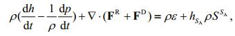 (1)
(1)where ρ is the in situ density, p is the pressure, h is the specific enthalpy (h=U+p/ρ, including the specific internal energy U, and the work done by pressure forces p/ρ), and d/dt=∂/∂t+v·∇ is the material derivative following the instantaneous fluid velocity v. The quantities in the divergence term are the nonadvective heat fluxes, including the sum of boundary and radiative heat fluxes FR at the ocean surface and sea floor, and molecular diffusive energy fluxes FD (IOC et al., 2010). The terms on the right-hand side of the equation specify interior sources, where ρε is a small term indicating the rate of dissipation of kinetic energy into thermal energy, and 
Similar to the definition of potential temperature, the potential enthalpy h0 is defined as the enthalpy a water parcel would have at a reference pressure pr (chosen to be at the sea surface, where pr=0 dbar in this paper) if raised in a reversible manner (isentropic, isohaline and without the dissipation of kinetic energy),
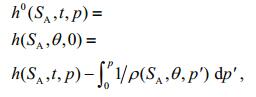 (2)
(2)where SA is the absolute salinity, t is the in situ temperature on the celsius (℃) scale, and θ is the potential temperature with respect to a reference pressure pr on the celsius scale.
The conservative temperature Θ is defined to be proportional to the potential enthalpy h0,
 (3)
(3)where Cp0 is a constant indicating the mean specific heat capacity between 0℃ and 25℃ at salinity of 35 (IOC et al., 2010),
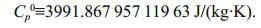 (4)
(4)Thus, Eq.1 can be simplified in terms of h0 or Θ to a very high accuracy (IOC et al., 2010; Graham and McDougall, 2013),
 (5)
(5)where T0=273.15 K is the temperature offset between Kelvins and degrees Celsius, and μ(p) is the relative chemical potential of salt in seawater (the difference of the partial chemical potential between salt and water) at pressure p. Equation 5 states that the values of h0 and Θ of a fluid parcel can change as a result of (1) the divergence of the flux of heat at the boundaries, (2) the dissipation of kinetic energy into thermal energy, (3) interior salinity sources caused by remineralization, and (4) a residual term associated with the chosen of the reference pressure pr, which is zero at the reference pressure pr. It can be seen that the quantities h0 and Θ are still not completely conserved because of the existence of the source terms ρε and
Using Gauss' divergence theorem, and ignoring the source terms 
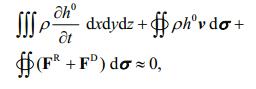 (6)
(6)or
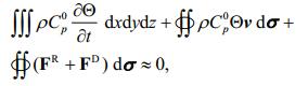 (7)
(7)where σ is the unit outward vector normal to the boundary σ. Equation 7 illustrates the temporal OHC variations influenced by heat sources/sinks at the boundaries. Compared with the total energy conservation equation, the evolution equation for mechanical energy is subtracted in Eqs.6, 7 to better illustrate the "heat" variations (IOC et al., 2010). Thus, the OMHT based on the fluxes of h0 does not include the transport of mechanical energy. In fact, the difference between the total energy transport, which is the flux of the Bernoulli function, and heat transport, which is the flux of h0, is only about 0.003℃ when expressed in temperature units, and can be ignored (McDougall, 2003).
Thus, the ocean heat content OHC is actually the volume integral of Θ
 (8)
(8)Note that the flux FR works on the ocean surface/ floor, so that an area integral over an ocean section is zero. Thus, the heat transport across a zonal ocean section OMHT is the sum of an advection term OMHTadv and a diffusion term OMHTdif
 (9)
(9)Where
 (10)
(10) (11)
(11)and n is the unit northward vector, so that a positive value of OMHT indicates a northward heat transport. The diffusion term OMHTdif is small unless near strong oceanic fronts, such as the Antarctic Circumpolar Circulation and the west boundary currents (Yang et al., 2015a). Here, Θ is calculated using Gibbs Seawater Oceanographic Toolbox Version 3.05.5 (McDougall and Barker, 2011), and the diffusion term is calculated based on parameterized model outputs.
Despite the non-conservation of the quantities h0 and Θ, the error by assuming h0 or Θ are perfectly conservative is approximately 120 times smaller than the corresponding error for potential temperature (McDougall, 2003; Graham and McDougall, 2013). Thus, we ignore the non-conservative aspect of the quantities h0 and Θ, and focus on the errors due to the neglect of the non-conservative production of potential temperature θ here. In the following, the error of a variable is the value calculated with potential temperature θ minus the value calculated with Θ, and specifies the error induced by the neglect of the nonconservation of the traditionally-used potential temperature.
3.2 Temperature errorThe temperature error (θ–Θ) as a function of absolute salinity SA and conservative temperature Θ is illustrated in Fig. 1. The temperature error is quite small when the temperature is close to 0℃ or salinity is close to 35 (McDougall, 2003; IOC et al., 2010). When the temperature is over 0℃ and the salinity is under 35, the potential temperature is smaller than the conservative temperature, and the temperature error becomes larger when the temperature increases or salinity decreases. The maximum temperature error reaches 1.8℃ when the water is extremely fresh and warm (around 40℃ and salinity of 0), which implies a large error near the coastal regions at mid-low latitudes. For high-salinity waters (> 35), the potential temperature is larger than the conservative temperature. While the temperature error becomes larger with increased salinity, the absolute error is not large, which suggests a slightly larger temperature error in the subtropical Atlantic than in the subtropical Pacific.

|
| Fig.1 Temperature error (potential temperature minus conservative temperature, θ−Θ) as a function of practical salinity and conservative temperature |
The spatial patterns of the error in sea surface temperature (SST) under modern and LGM climate conditions are very similar (Fig. 2). In both simulations, the temperature error and its standard deviation are most significant in the regions where the warm, fresh river runoffs discharge into the ocean, such as the Amazon estuary and the East China Sea. In these regions, the temperature error reaches 0.9℃ and the standard deviation of an annual cycle reaches 0.3℃. Thus, as the non-conservative temperature production cannot be ignored, the conservative temperature should be used instead of the potential temperature when analyzing processes associated with "heat" in the coastal regions, such as the heat content, heat advection, and surface heat fluxes. In the oceans away from the coast, the temperature error is small. At high latitudes where the main thermocline outcrops, the local temperature is close to 0℃, and the temperature error is very small (typically < 0.02℃), with negligible monthly fluctuations (typically < 0.01℃). In the subtropical gyres where the local salinity is very high (typically > 35), the potential temperature exceeds the conservative temperature by ~0.02℃ in the Pacific and ~0.04℃ in the Atlantic, and the monthly fluctuations are also very small (typically < 0.01℃). In the modern (LGM) simulation, the surface salinity in the subtropical gyre is typically 34.87 (35.06) in the North Pacific and 36.27 (37.06) in the North Atlantic Ocean. Consequently, the temperature error is much larger in the Atlantic because of the high salinity. In the warm-pool regions near the equator, the potential temperature is smaller than the conservative temperature by ~0.06℃ in the modern simulation and ~0.04℃ in the LGM simulation. The monthly fluctuations of the temperature error are also larger in the warm-pool regions on the order of 0.01℃.

|
| Fig.2 Annual mean (a, c) and standard deviation (b, d) of the climatological monthly mean temperature differences (θ−Θ) at the sea surface in the modern (a, b) and LGM (c, d) simulations The sea level was ~120-130 m lower during the LGM. Map drawing No. GS(2016)1611 (accessed from the National Administration of Surveying, Mapping and Geoinformation of China). |
In the ocean interior, the temperature error mainly appears along the main thermocline (Fig. 3), above which the potential temperature is smaller than the conservative temperature in the warm-pool regions in the Pacific, and this pattern extends to a depth of about 100 m (see Fig. 3a, c). In the main thermocline, the potential temperature exceeds the conservative temperature by 0.01℃ (0.02℃) along 180°E, and 0.03℃ (0.05℃) along 30°W in the modern (LGM) simulation. The subtropical temperature error under the LGM climate conditions is much larger than the error under modern climate conditions, because of the existence of continental ice sheets, which induced much saltier oceans during the LGM. The maximum temperature error appears in the salty subtropical Atlantic around 30°N, reaching up to 0.08℃. Below the main thermocline, the temperature is near 0℃ and the temperature error is smaller than 0.01℃.

|
| Fig.3 Annual mean conservative temperature Θ (contours at 3℃ intervals) and the temperature error (θ−Θ, color shading in ℃) along 180°E in the Pacific (a, c) and 30°W in the Atlantic (b, d) in the modern (a, b) and LGM (c, d) simulations |
The temperature errors over the past 22 000 years are illustrated in Fig. 4 based on the TraCE-21ka project. Consistent with the modern and LGM simulations, large temperature errors mainly appear in the mid-low latitudes, especially in the warm-pool regions and subtropical gyres. In the warm-pool regions, the potential temperature is smaller (typically 0.04℃) than the conservative temperature at the sea surface (Fig. 4a), but this pattern does not penetrate very deeply. The potential temperature becomes larger than the conservative temperature at a depth of 150 m, and the temperature error (almost) vanishes (< 0.02℃) at 600 m depth. In the subtropical gyre, the potential temperature is larger than the conservative temperature. In the subtropical gyre, the potential temperature at the sea surface is larger by about 0.02 and 0.04℃ than the conservative temperature in the Pacific and the Atlantic, respectively. This temperature difference decreases with increasing depth.

|
| Fig.4 Historical mean (a–c) and standard deviation (d–f) of the decadal annual mean temperature differences (θ−Θ) at depths of 5 m (a, d), 150 m (b, e) and 600 m (c, f) over the past 22 000 years based on the TraCE-21ka outputs Map drawing No. GS(2016)1611 (accessed from the National Administration of Surveying, Mapping and Geoinformation of China). |
The historical fluctuations of the temperature error are most significant in the warm-pool regions and subtropical North Atlantic, and peaks vertically near the surface (Fig. 4d–f). In the modern and LGM simulations, the standard deviations of the climatological monthly mean surface temperature errors in the North Atlantic are less than 0.01℃, suggesting small monthly fluctuations (see Fig. 2b, d). In the TraCE-21ka project, however, the historical standard deviation is up to 0.05℃ in the subtropical North Atlantic (Fig. 4d), which may be related to the significant climate change in the North Atlantic over the past 22 000 years. The standard deviation decreases with increasing depth. At 150 m depth, it is typically 0.01℃ in the North Atlantic subtropical gyre and < 0.01℃ elsewhere.
3.3 The error in heat contentThe OHC is traditionally calculated based on the potential temperature θ using 

|
| Fig.5 Global (black), Pacific plus Indian (red) and Atlantic (blue) OHC (a, c) and the OHC error (b, d) integrated in each 10° latitude band in the modern (a, b) and LGM (c, d) simulations The OHC is calculated based on Eq.8 and the OHC error is the heat content calculated based on the traditionally-used potential temperature minus the value based on conservative temperature. The total heat content (error) for the entire meridional range is labeled in the top right corner with corresponding colors. |
The relative OHC error over the past 22 000 years is dominated by the robust OHC variations (see Fig. 6). The absolute changes of the OHC errors themselves are minor, but the OHC became one order of magnitude larger over the past 22 000 years. In the most recent glacial cycle, the ice sheets reached their greatest extent during the LGM at ~21 ka, covering North America north of the Great Lakes and northern Eurasia at a thickness up to 4.5 km (Peltier, 2004). The LGM is a relatively steady climate state with a consistent magnitude of the OHC. The ice sheets began to retreat at ~20 ka (Toucanne et al., 2009), and the melting water raised the sea level by ≈120 m in the following glacial termination (Denton et al., 2010). The OHC increased roughly 6-fold during this period (Fig. 6a). At ~7 ka, the North American ice sheets almost vanished (Dyke and Prest, 1987; Kleman et al., 2010), marking the onset of the Holocene, after which the heat content became steady again. Overall, the relative OHC error decreased rapidly from 1.49% to 0.27% between the LGM and the modern era, and almost all reductions occurred at the last glacial termination roughly between 20 ka and 7 ka in the TraCE-21ka simulation.

|
| Fig.6 Time series of OHC (a), the OHC error (b) and the relative OHC error (c) over the past 22 000 years based on the TraCE-21ka outputs |
The OMHT can be divided into an advection term and a much smaller molecular diffusion term. The advective OMHT is traditionally calculated based on potential temperature θ using 

|
| Fig.7 Annual mean OMHT (a, c) and the OMHT error (b, d) for the global (black), Pacific plus Indian (red), and Atlantic (blue) basins in the modern (a, b) and LGM (c, d) simulations The OMHT is calculated based on Eq.9. The OMHT error is the OMHT calculated based on the traditionally-used potential temperature minus the value based on conservative temperature. |
The patterns of the OMHT are very similar under the modern and LGM climate conditions (Fig. 7), which is dominated by the direct advection of water parcels with difference conservative temperature (Yang et al., 2015a). In the Pacific plus Indian basins, heat is transported away from the tropics to mid-high latitudes, but the transport strength is weak in the subpolar regions. The OMHT is dominated by the shallow wind-driven thermohaline subtropical cells confined to the tropics and subtropics. The warm water in the upper ocean is transported poleward by the surface winds and the western boundary currents and returns with a reduced conservative temperature (described in terms of the potential temperature in previous articles) in the ocean interior (McCreary Jr and Lu, 1994; Gu and Philander, 1997). In the Atlantic, heat is transported from the south to the north in both hemispheres and its strength is still robust at high latitudes. The OMHT in the Atlantic is dominated by the deep thermohaline circulation because of the formation of the North Atlantic Deep Water (NADW). Warm water in the upper ocean flows northward and returns as cold NADW in both hemispheres (Bryden and Imawaki, 2001; Ferrari and Ferreira, 2011; Macdonald and Baringer, 2013). The temperature difference is large (typically 10℃) and the strength of the overturning is strong (typically 18 Sv). Consequently, this deep circulation carries the heat of about 0.8 PW and hence dominates the OMHT in the Atlantic Ocean (Bryden and Imawaki, 2001). The subtropical cells also have effects in the Atlantic, so that the northward heat transport in the northern hemisphere is much larger than that in the southern hemisphere. For the global ocean, the OMHT is poleward, and the ocean generally acts to compensate the tropical surplus and polar deficit in energy at the top of the atmosphere (Hatzianastassiou et al., 2004).
The OMHT error in the LGM climate is almost identical to the error in the modern climate, with a difference < 0.001 PW (Fig. 7; 1 PW=1015 W). The pattern of the OMHT error is dominated by surface temperature errors (see Fig. 3). The pattern of the OMHT error is determined by the temperature error near the surface. In the Atlantic Oceans as well as the subtropical gyres in the Pacific Ocean and the Indian Ocean, the potential temperature is larger than the conservative temperature (see Fig. 2a, c), and the OMHT there is overestimated if using potential temperature (Fig. 7b, d). In the low-latitude warm pool regions, however, the conservative temperature is larger and the OMHT there are underestimated (Fig. 7b, d). Overall, the pattern of the global OMHT error is dominated by the Indo-Pacific OMHT error, just as the pattern of the global OMHT is dominated by the Indo-Pacific OMHT (Fig. 7), which is typically < 0.005 PW, with a maximum of 0.007 PW for the global ocean, and induces a typical OMHT relative error of ~0.3% under both the modern and LGM climate conditions.
The patterns of the OMHT and OMHT errors are consistent with the patterns from the modern and LGM simulations (Fig. 8). In the Indo-Pacific Ocean or even worldwide, the OMHT is poleward. The use of the potential temperature overestimates the OMHT at mid-latitudes and underestimates it near the equator. In the Atlantic, the OMHT is northward in both hemispheres, and is overestimated by the use of potential temperature. In contrast to the significant changes in historical OHC, the OMHT and OMHT errors were relatively steady over the past 22 000 years. The mean range (maximum minus minimum) of the OMHT over the past 22 000 years is about 0.35 PW, and the value of the OMHT error is 0.002 PW. The mean fluctuations (standard deviation) of the historical OMHT error is 0.000 4 PW, which suggests that the temporal variations of the OMHT error can be ignored to a very high accuracy.

|
| Fig.8 Time averaged (solid line) and range (maximum and minimum, shading) of global (a), Pacific plus Indian (b), and Atlantic (c) OMHT over the past 22 000 years based on TraCE-21ka simulations; (d–f) as in (a–c), but for the OMHT error |
The energy budgets of the ocean require a conservative quantity, whose changes are determined by external heat forcing at the boundaries, irrespective of interior processes. The potential temperature is traditionally used as the required conservative quantity, but it is usually affected by turbulent mixing. The quantities that can be conserved during mixing at a constant pressure are mass, salt, and enthalpy (Fofonoff, 1962). Enthalpy is related to the energy of the ocean, but it cannot be used directly as the required conservative quantity because it also depends on vertical motion. Thus, similar to the definition of potential temperature, potential enthalpy and conservative temperature are proposed (McDougall, 2003), since they are two orders of magnitude more conservative than potential temperature, and are the quantities more closely related to the advection and diffusion of "heat" (McDougall, 2003; IOC et al., 2010).
The conservative temperature should be used to express ocean processes associated with "heat" instead of the traditionally-used potential temperature, because the error resulting from the neglect of the non-conservation of potential temperature is generally < 1% when analyzing basin-scale ocean processes. The error is at least one order of magnitude smaller than the model bias, but we insist that the quantified errors are reliable. We all agree that we cannot use energy conservation to estimate the errors, because of the model bias and the errors of approximations. Instead, our calculations are based on the patterns of ocean temperature and velocity. Thus, a typical 10% model bias will induce a similar magnitude of fluctuation of our estimations, and will not induce significant influences on the conclusions. A similar method has been applied by Macdonald and Baringer (2013) to estimate the error of the OMHT in the modern climate, and we have further quantified the errors of both the OHC and OMHT in simulations carried out for the past 22 000 years.
5 CONCLUSIONBased on climatological simulations under modern and LGM climate conditions, and a transient simulation of the past 22 000 years, we have quantified the errors due to the neglect of the non-conservation of potential temperature. The temperature error reaches 0.9℃ with strong monthly variations near the coast, especially in the regions with warm and fresh river discharges. In the open oceans, the temperature error is small, mainly appears along the main thermocline, and is much larger (typically 0.03℃) in the mid-low latitudes above the main thermocline. At high latitudes where the main thermocline outcrops, as well as in the regions below the main thermocline, the temperature error is generally < 0.01℃. The associated OHC error is on the order of 3×10²² J, corresponding to roughly the 5–7 year increment of the upper 1 500 m OHC resulting from increases in greenhouse-gas concentrations (Chen and Tung, 2014). The OHC error is relatively steady over the past 22 000 years, but the OHC in the modern climate is about six times the value in the LGM climate. Thus, the percentage of the OHC error decreases from 1.2% in the LGM climate to 0.14% in the modern climate, with the main decrease occurring during the last glacial termination roughly from 20 ka to 7 ka. The associated OMHT error is typically < 0.005 PW. The temporal variations of the OMHT error are also very small, with the mean standard deviation of the historical OMHT error over the past 22 000 years only about 0.000 4 PW. Generally speaking, the relative OMHT error over the past 22 000 years is 0.3%. Overall, the error induced by the neglect of the non-conservation of potential temperature induces a small (generally < 1%) relative error with respect to the calculation of OHC and OMHT when analyzing basin-scale climate variations. This suggests that the calculations based on conservative temperature can be compared directly with previous calculations based on potential temperature, but the difference should also be noted for more accurate model simulations in the future.
6 DATA AVAILABILITY STATEMENTThe transient TraCE-21ka databases are available from ftp://pike.aos.wisc.edu by using the public account with username: ccrguest and password: Climate.
The modern experiment is the case b30.030a from 20C3M (20C3M run1), and the LGM experiment is the case b30.104w from PMIP2. Both of the databases are available from the website of the Earth System Grid https://www.earthsystemgrid.org after registration.
7 ACKNOWLEDGEMENTWe thank the National Center for Atmospheric Research (NCAR), the Earth System Grid Federation (ESGF) and University of Wisconsin-Madison for sharing the data with the public. We thank YANG Haijun, LI Qing and WANG Kun from Beijing University for assistance in the calculations of heat transport. All the calculations involving potential enthalpy and conservative temperature are calculated using Gibbs-SeaWater (GSW) Oceanographic Toolbox Version 3.05.5 in Matlab, and we thank Trevor J. McDougall and Paul M. Barker for their efforts. We also thank two anonymous reviewers, GUO Yongqing, ZHANG Cong and DUAN Juan for their efforts to improve the quality of the article. We thank Richard Foreman, PhD, from Liwen Bianji, Edanz Editing China (www.liwenbianji.cn/ac), for editing the English text of a draft of this manuscript.
Batchelor G K. 1967. An Introduction to Fluid Dynamics. Cambridge University Press, Cambridge. 615p.
|
Bryan K. 1962. Measurements of meridional heat transport by ocean currents. Journal of Geophysical Research, 67(9): 3 403-3 414.
DOI:10.1029/JZ067i009p03403 |
Bryden H L, Imawaki S. 2001. Ocean heat transport. In: Siedler G, Church J, Gould J eds. Ocean circulation and climate: Observing and Modelling the Global Ocean.Academic Press, San Fransisco CA, USA. p.455-474.
|
Chen X, Tung K K. 2014. Climate. Varying planetary heat sink led to global-warming slowdown and acceleration. Science, 345(6199): 897-903.
|
Denton G H, Anderson R F, Toggweiler J R, Edwards R L, Schaefer J M, Putnam A E. 2010. The last glacial termination. Science, 328(5986): 1 652-1 656.
DOI:10.1126/science.1184119 |
Dyke A S, Prest V K. 1987. Late Wisconsinan and Holocene history of the Laurentide ice sheet. Géographie Physique et Quaternaire, 41(2): 237-263.
DOI:10.7202/032681ar |
Ferrari R, Ferreira D. 2011. What processes drive the ocean heat transport?. Ocean Modelling, 38(3-4): 171-186.
DOI:10.1016/j.ocemod.2011.02.013 |
Fischer N, Jungclaus J H. 2010. Effects of orbital forcing on atmosphere and ocean heat transports in Holocene and Eemian climate simulations with a comprehensive Earth system model. Climate of the Past, 6(2): 155-168.
DOI:10.5194/cp-6-155-2010 |
Fofonoff N. 1962. Physical properties of sea-water. The Sea, 1: 3-30.
|
Gill A E. 1982. Atmosphere-Ocean Dynamics. Academic Press, New York. 662p.
|
Graham F S, McDougall T J. 2013. Quantifying the nonconservative production of conservative temperature, potential temperature, and entropy. J. Phys. Oceanogr., 43(5): 838-862.
DOI:10.1175/JPO-D-11-0188.1 |
Gu D F, Philander S G H. 1997. Interdecadal climate fluctuations that depend on exchanges between the tropics and extratropics. Science, 275(5301): 805-807.
DOI:10.1126/science.275.5301.805 |
Hatzianastassiou N, Matsoukas C, Hatzidimitriou D, Pavlakis C, Drakakis M, Vardavas I. 2004. Ten year radiation budget of the Earth:1984-93. International Journal of Climatology, 24(14): 1 785-1 802.
DOI:10.1002/(ISSN)1097-0088 |
He F. 2011. Simulating Transient Climate Evolution of the Last Deglaciation with CCSM3. University of WisconsinMadison, Wisconsin. 171p.
|
IOC, SCOR, IAPSO. 2010.The international thermodynamic equation of seawater-2010: calculation and use of thermodynamic properties. In: Intergovern-mental Oceanographic Commission, Manuals and Guides No. 56. Paris: IOC, SCOR, IAPSO, 196.
|
IPCC. 2007. Climate Change 2007: Synthesis Report.Contribution of Working Groups I, Ⅱ and Ⅲ to the Fourth Assessment Report of the Intergovernmental Panel on Climate Change. Intergovernmental Panel on Climate Change, Cambridge. 104p.
|
Jackson L C, Kahana R, Graham T, Ringer M A, Woollings T, Mecking J V, Wood R A. 2015. Global and European climate impacts of a slowdown of the AMOC in a high resolution GCM. Climate Dynamics, 45(11-12): 3 299-3 316.
DOI:10.1007/s00382-015-2540-2 |
Kleman J, Jansson K, De Angelis H, Stroeven A P, Hättestrand C, Alm G, Glasser N. 2010. North American Ice Sheet build-up during the last glacial cycle, 115-21 kyr. Quaternary Science Reviews, 29(17-18): 2 036-2 051.
DOI:10.1016/j.quascirev.2010.04.021 |
Macdonald A M, Baringer M O. 2013. Ocean heat transport. International Geophysics, 103: 759-785.
DOI:10.1016/B978-0-12-391851-2.00029-5 |
Marschall J, Plumb R A. 2008. Atmosphere, Ocean, and Climate Dynamics. Elsevier Academic Press, Burlington. 344p.
|
Marson J M, Wainer I, Mata M M, Liu Z. 2014. The impacts of deglacial meltwater forcing on the South Atlantic Ocean deep circulation since the Last Glacial Maximum. Climate of the Past, 10(5): 1 723-1 734.
DOI:10.5194/cp-10-1723-2014 |
McCreary Jr J P, Lu P. 1994. Interaction between the subtropical and equatorial ocean circulations:the subtropical cell. J.Phys. Oceanogr., 24(2): 466-497.
DOI:10.1175/1520-0485(1994)024<0466:IBTSAE>2.0.CO;2 |
McDougall T J, Barker P M. 2011. Getting started with TEOS-10 and the Gibbs Seawater (GSW) oceanographic toolbox. SCOR/IAPSO WG, 127: 1-28.
|
McDougall T J. 2003. Potential enthalpy:a conservative oceanic variable for evaluating heat content and heat fluxes. J Phys Oceanogr, 33: 945-963.
DOI:10.1175/1520-0485(2003)033<0945:PEACOV>2.0.CO;2 |
Olbers D, Willebrand J, Eden C. 2012. Ocean dynamics.Springer, Heidelberg. 704p.
|
Otto-Bliesner B L, Brady E C, Clauzet G, Tomas R, Levis S, Kothavala Z. 2006. Last glacial maximum and Holocene climate in CCSM3. Journal of Climate, 19(11): 2 526-2 544.
DOI:10.1175/JCLI3748.1 |
Peltier W R. 2004. Global glacial isostasy and the surface of the ice-age earth:the ICE-5G (VM2) model and GRACE. Annual Review of Earth and Planetary Sciences, 32(1): 111-149.
DOI:10.1146/annurev.earth.32.082503.144359 |
Stouffer R J, Yin J, Gregory J M, Dixon K W, Spelman M J, Hurlin W, Weaver A J, Eby M, Flato G M, Hasumi H, Hu A, Jungclaus J H, Kamenkovich I V, Levermann A, Montoya M, Murakami S, Nawrath S, Oka A, Peltier W R, Robitaille D Y, Sokolov A, Vettoretti G, Weber S L. 2006. Investigating the causes of the response of the thermohaline circulation to past and future climate changes. Journal of Climate, 19(8): 1 365-1 387.
DOI:10.1175/JCLI3689.1 |
Tailleux R. 2015. Observational and energetics constraints on the non-conservation of potential/conservative temperature and implications for ocean modelling. Ocean Modelling, 88: 26-37.
DOI:10.1016/j.ocemod.2015.02.001 |
Toucanne S, Zaragosi S, Bourillet J F, Cremer M, Eynaud F, Van Vliet-Lanoë B, Penaud A, Fontanier C, Turon J L, Cortijo E. 2009. Timing of massive 'Fleuve Manche' discharges over the last 350 kyr:insights into the European ice-sheet oscillations and the European drainage network from MIS 10 to 2. Quaternary Science Reviews, 28(13-14): 1 238-1 256.
DOI:10.1016/j.quascirev.2009.01.006 |
Trenberth K E, Fasullo J T. 2013. An apparent hiatus in global warming?. Earth's Future, 1(1): 19-32.
DOI:10.1002/2013EF000165 |
Warren B A. 1999. Approximating the energy transport across oceanic sections. Journal of Geophysical Research:Oceans, 104(C4): 7 915-7 919.
DOI:10.1029/1998JC900089 |
Yang H J, Li Q, Wang K, Sun Y, Sun D. 2015a. Decomposing the meridional heat transport in the climate system. Climate Dynamics, 44(9-10): 2 751-2 768.
DOI:10.1007/s00382-014-2380-5 |
Yang H J, Zhao Y Y, Liu Z Y, Li Q, He F, Zhang Q. 2015b. Heat transport compensation in atmosphere and ocean over the past 22, 000 years. Sci. Rep., 5: 16 661.
DOI:10.1038/srep16661 |
Zhang R, Delworth T L. 2005. Simulated tropical response to a substantial weakening of the Atlantic thermohaline circulation. Journal of Climate, 18(12): 1 853-1 860.
DOI:10.1175/JCLI3460.1 |