 2019, Vol. 37
Institute of Oceanology, Chinese Academy of Sciences
Article Information
- LÜ Xianqing, WANG Daosheng, YAN Bing, YANG Hua
- Coastal sea level variability in the Bohai Bay: influence of atmospheric forcing and prediction
- Journal of Oceanology and Limnology, 37(2): 486-497
- http://dx.doi.org/10.1007/s00343-019-7383-y
Article History
- Received Dec. 14, 2017
- accepted in principle Feb. 8, 2018
- accepted for publication Jul. 2, 2018


2 Physical Oceanography Laboratory/CIMST, Ocean University of China and Qingdao National Laboratory for Marine Science and Technology, Qingdao 266100, China;
3 College of Marine Science and Technology, China University of Geosciences, Wuhan 430074, China;
4 Shenzhen Research Institute, China University of Geosciences, Shenzhen 518057, China
Understanding the dynamics in the regions of coastal waters is considered to be very important not only in the hydrodynamic sense but also in the study of biologic productivity and water quality (Paraso and Valle-Levinson, 1996; Sun et al., 2015). For example, the harbors are traditionally constructed in the coastal areas, so the prediction of coastal sea level (SL) variability can help navigation in shallow waters.
The coastal total SL is composed of several components, including the mean SL, the tides, the SL affected by the sea surface atmospheric pressure (AP), the dynamic adjustment of SL to wind-driven currents, eddies and coastally trapped waves, steric SL variations associated with the seawater thermal expansion on seasonal to climatic temporal scales, and so on (Kurapov et al., 2017). The globally averaged change in mean SL is on the order of 0.001 m/yr (Chen et al., 2017; Quartly et al., 2017). The seasonal variation of the SL associated with the seawater thermal expansion is about 0.01 m (Mellor and Ezer, 1995). The tidal SL can be obtained from the Oregon State University Inverse Tidal Software (OTIS; Egbert and Erofeeva, 2002) and other global tidal models (e.g., Le Provost et al., 1998; Matsumoto et al., 2000; Cheng and Andersen, 2011). The SL affected by the sea surface AP can be calculated using the inverted barometer correction (IB; Paraso and Valle-Levinson, 1996); nevertheless, the ocean response to AP is farther from the classical IB response in the shallow and coastal areas (Carrère and Lyard, 2003; Carrere et al., 2016).
Besides, the wind-driven SL variabilities are different in studies on diverse areas and timescales. Sandstrom (1980) showed that the SL changes were highly correlated with variations in the alongshore component of wind by analyzing the coastal tide gage records and coincident weather data. Hsueh and Romea (1983) analyzed the low-pass (< about 0.85 cpd) filtered coastal SL data and geostrophic winds, and found that SL fluctuations along the west coast of Korea were highly coherent with the northsouth wind. Zhao and Cao (1987) analyzed the low frequency (< 0.59 cpd) fluctuations of the wintertime coastal SL in the Yellow Sea and East China Sea, based on the pressure, wind and SL data at nine coastal stations. They found that the principal direction of wind inducing fluctuation of the SL in the Yellow Sea and Northern East China Sea was about NNW-SSE direction, which was almost the same as the stretching of Korea Peninsula and Yellow Sea Trough. Castro and Lee (1995) found that SL fluctuations in the central and northern portions of the South Brazil Bight for both 9- to 12- and 6- to 7-day bands were better correlated with winds located southward and earlier in time than with the local wind at the time of SL measurement. Andres et al. (2013) found that local along-shelf wind stress was an important driver of coastal SL variability at interannual time and remote forcing may also be important both at interannual time scales and at lower frequencies. Thompson et al. (2014) pointed out that the predictability of decadal SL change rates along the northeast Pacific coastline was largely determined by tropical variability, rather than longshore wind stress and local winds stress curl. Piecuch et al. (2016) highlighted the importance of barotropic dynamics on coastal SL changing on the interannual and decadal time scales.
The observations of SL used in the aforementioned and many other studies were near the continental shelfs or deep waters. Li and Yang (1983) used stochastic process theory to make a spectral analysis of the SL, wind stress and AP at the Bohai Bay, which is a typical semi-enclosed coastal sea and has limited water exchange with the ocean (Meng et al., 2008), and found that the relationship between the SL and the atmospheric forcing was linear, but they did not predict the SL variability. Liu et al. (2017) used tide gauge data, from 1950 to 2015, to evaluate the sea level rise in the Bohai Bay and associated responses. In this paper, the observed SL and coincident observations of atmospheric forcing, at two stations located in the Bohai Bay, were used to analyze the relationship between SL and atmospheric forcing, including AP and local winds, which was then utilized to predict the SL variability. In the Bohai Bay that is a shallow shelf sea, there is no significant steric variations that could produce geostrophic currents, so the ocean current features will not be discussed in this study. The rest of this paper is structured as follows: the observations of SL, AP and wind were described in Section 2; in Section 3, the relationship between SL and atmospheric forcing was analyzed, and then the total SL was predicted; the discussions and conclusions can be found in Sections 4 and 5, respectively.
2 OBSERVATIONObservations used in the following analysis were obtained from two stations (E1 and E2) located in the Bohai Bay (Fig. 1). Because that the Bohai Bay is a shallow shelf sea (Fig. 1), there is no significant height changes associated with geostrophic currents. Besides, there are prominent hills nearby, so the winds are not constrained by the land topography. At each station, the total SL, the 10 m wind and the sea level AP were observed hourly. The total SLs, at E1 and E2, were measured using the moored pressure gauge, which was accurate to within 5 cm. The undisturbed depth at E1 and E2 was about 3.3 m and 15.7 m, respectively. The 10 m wind and sea level AP were measured using the XZY3-type automatic observing system, in which the 10 m wind was measured by the XFY3-1 propeller anemograph, which was accurate to within 5° for wind direction and 0.5 m/s for wind speed. The duration of the observation is 91 days (from 0000 UTC 19 August 2014 to 0000 UTC 18 November 2014) with continuous coverage.

|
| Fig.1 General location of the Bohai Sea (rectangle with dashed lines) (a); locations (denoted by black stars) of the observation stations, E1 and E2, in the Bohai Bay, and the bathymetric contours at 10 m and 40 m (b) |
The power spectral densities of the observed total SL, u wind component and v wind component at E1 and E2 were calculated and shown in Fig. 2 and Fig. 3, respectively. At both E1 and E2, the SL fluctuations were dominated by the motions in the semidiurnal frequency band, suggesting that the semidiurnal tides were the most energetic. Additional significant spectral peaks appeared in the diurnal frequency band, showing that the diurnal tides were the second energetic motions. Besides, there were spectral peaks at frequencies of the higher harmonics, because of nonlinear interaction and advection of the main diurnal and semidiurnal tides (Xu et al., 2013). At E1, the u wind component and v wind component were dominated by motions in the diurnal frequency band, while there was an additional significant spectral peak near the inertial band for the v wind component, which was about 1.33 cpd, with a blue shift of about 7.3% above the inertial frequency at E1 (1.24 cpd) (Garrett, 2001). On the contrary, there were two significant spectral peaks in the power spectral density of the u wind component at E2, which were in the diurnal and semidiurnal bands, respectively. Besides the significant peak in the diurnal frequency in the power spectral density of the v wind component at E2, there was a nearly significant spectral peak near the inertial band (1.25 cpd), which was about 1.23 cpd.

|
| Fig.2 The power spectral densities of the observed SL (red line) and LSL (blue line) (a), the observed u wind component (red line) (b), and the observed v wind component (red line) (c), at E1 In all the panels, the red and blue dashed lines designate the corresponding 5% significance level against red noise. The diurnal (D1) and semidiurnal (D2) frequency bands are shown by gray shades in all the panels, and the black dashed lines in (b) and (c) show the inertial frequency at E1. |

|
| Fig.3 Same as Fig. 2 but for those at E2 |
The hourly observed SLs were filtered using a cosine-lanczos filter with a high frequency cut-off of 0.8 cpd, through which the tidal, local inertial and higher frequency signals were eliminated, and the low-pass result was labelled as LSL. The power spectral densities of LSL at E1 and E2 were calculated and shown in Fig. 2a and Fig. 3a, respectively. It was obvious that the high frequency cut-off performed for LSL at both E1 and E2 were effective. In the power spectral density of LSL at E1, several significant peaks appeared from about 1.8-day period to 3.6-day period. Similarly, the significant high energies at E2 appeared in a band with periods of from 1.7 to 3.8 days for LSL.
Similar to Sandstrom (1980), Hsueh and Romea (1983), and Castro and Lee (1995), all the observations at E1 and E2, including the LSL, u wind, v wind and AP, were sub-sampled from hourly to 6-hourly intervals. The sub-sampled LSL was labelled as SLSL, while SUW, SVW, SW and SAP for the subsampled u wind, v wind, wind and AP, respectively. The time series of SLSL, SUW, SVW and SAP, at both E1 and E2, were shown in Fig. 4.

|
| Fig.4 Time series of SLSL and SAP (a), SUW (b) and SVW (c), at E1 and E2 |
As shown in Fig. 4a, SLSLs at E1 and E2 were almost equal with those at E1 being sometimes slightly larger. The mean and standard deviation for SLSLs at E1 were 0.10 m and 0.26 m, respectively, and those at E2 were 0.08 m and 0.25 m, which agreed with the qualitative results from Fig. 4a. The continuous wavelet power spectra (Grinsted et al., 2004) of SLSLs at E1 and E2 were shown in Fig. 5a and 5b, respectively. There were clearly common features in the wavelet power of these two SLSLs. Both SLSLs had high power in the 1.1–4.4 day band during 263–321 days related to 0000 UTC 1 January 2014 and in the 1.5–3.5 day band during 242–249 days related to 0000 UTC 1 January 2014. The cross wavelet power and phase (Grinsted et al., 2004) between SLSL at E1 and that at E2 were shown in Fig. 5c. It was noticed that the common features in the individual wavelet power spectra stood out as being significant at the 5% level. The cross wavelet transform also showed that SLSLs at E1 and E2 were in phase in all the sectors. The squared wavelet coherence and phase (Grinsted et al., 2004) between SLSL at E1 and that at E2 were shown in Fig. 5d. These two SLSLs showed high coherency and were in phase within the 5% significant regions, indicating that they were almost equal as illustrated by Fig. 4a.

|
| Fig.5 The continuous wavelet power of SLSL at E1 (a) and E2 (b); the cross wavelet power (contours) and phase (vectors) between SLSL at E1 and that at E2 (c); and the wavelet coherence (contours) and phase (vectors) between SLSL at E1 and that at E2 (d) In all the panels, the thick contour designates the 5% significance level against red noise and the cone of influence where edge effects might distort the picture is shown as a white blank. |
SUWs at E1 and E2 were just similar near several local extrema (Fig. 4b). The mean and standard deviation for SUW at E1 were -0.64 m/s and 2.14 m/s, respectively, and those at E2 were -0.06 m/s and 4.52 m/s, indicating that the fluctuations of SUW at E2 were larger than those at E1. The SVWs at E1 and E2 were more similar during the observational period (R=0.67), and the fluctuations of SVW at E2 were larger than those at E1 (Fig. 4c), as the standard deviations were 5.15 m/s and 2.35 m/s at E2 and E1, respectively. The fluctuations of both SUW and SVW at E2 were larger than those at E1, which may be related with that E1 was much closer to the land than E2.
3.2 Prediction of SLSLThe SLSL was influenced by the AP and wind, but there is no certain formula to calculate the relationships. To predict the SLSL, three methods were carried out, as follows:
(1) Multivariable linear regression model
In the multivariable linear regression model, the SLSL was assumed to be a linear combination of AP and wind, as follows:
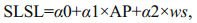 (1)
(1)where, ws is the wind component at the dominant wind orientation; α0, α1 and α2 are the regression coefficients.
(2) Linear regression model
In the linear regression model, the SLSL was assumed to be a linear function of the wind at the corresponding dominant wind orientation, as follows:
 (2)
(2)where, β0 and β1 are the regression coefficients.
(3) Linear regression model and IB
In this method, the SLSL influenced by AP was assumed to satisfy the classic IB relationship; besides, the ocean response to wind was linear. So, the SLSL can be calculated as follows:
 (3)
(3)where, SLSL_IB is the SL affected by AP, which can be calculated through the IB formulate as shown in Paraso and Valle-Levinson (1996) and Kurapov et al. (2017); ASLSL is the adjusted SLSL, which is equal to the SLSL minus the SLSL_IB; γ0 and γ1 are the regression coefficients.
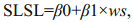
To find the dominant wind orientation influencing SLSL (ASLSL), the magnitude squared coherences between SLSL (ASLSL) and SW were calculated as functions of frequency and wind orientation measured clockwise from north at an interval of 5 degrees, which were shown in Fig. 6a (Fig. 6c) and Fig. 6e (Fig. 6g) for E1 and E2, respectively. In addition, the averaged values of the magnitude squared coherences at each wind orientation were also calculated, which were shown in Fig. 6b (Fig. 6d) and Fig. 6f (Fig. 6h) for E1 and E2, respectively.

|
| Fig.6 Contours of magnitude squared coherence between SLSL and SW at E1 as a function of frequency and wind orientation (in degree measured clockwise from north at an interval of 5 degrees) (a); the averaged values of the magnitude squared coherence between SLSL and SW at E1 at every wind orientation (b); (c–d) same as (a–b) but for those between ASLSL and SW at E1; (e–h) same as (a–d) but for those at E2 In (a): the black dashed contours connect values of 0.5, the red and magenta solid contours 0.7 and 0.9, and the locations of the maximum values are denoted by green star. Blue dotted lines in (a) and (b) show the wind orientation, where the averaged values reach the maximum. |
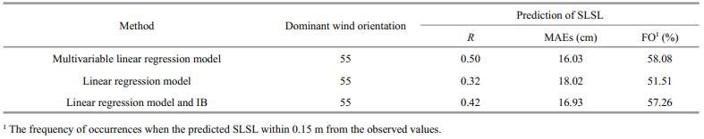
For the magnitude squared coherences between SLSL and SW at E1 (Fig. 6a), one coherent band was the most evident, in which the values were greater than 0.9 at about 2.6–2.8 days when the wind orientation was 25°–70°. In this evident coherent band, the maximum coherences were 0.93 (Table 1). Overall, the averaged values of the magnitude squared coherences reached the maximum value (0.35) when the wind orientation was 65° (Fig. 6b and Table 1), showing that SLSL at E1 was dominantly influenced by SW at 65°. The pattern of the magnitude squared coherences between ASLSL and SW at E1 (Fig. 6c) was obviously similar to those between SLSL and SW at E1 (Fig. 6a), in which the locations of the local maximum coherences were the same (Table 1). Besides, the ASLSL at E1 was dominantly influenced by SW at 70°(Fig. 6d and Table 1). Both the SLSL and ASLSL at E2 were dominantly influenced by SW at 55° (Fig. 6f, 6h and Table 1), which were different from those at E1.
|
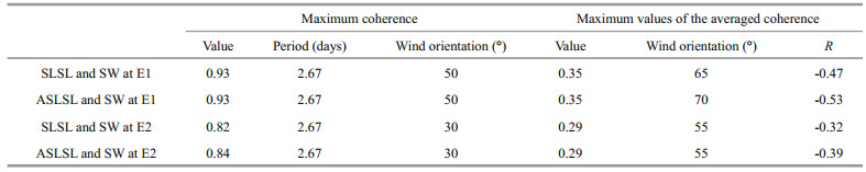
Based on the dominant wind orientation influencing SLSL (Table 1), the multivariable linear regression model (Eq.1) and linear regression model (Eq.2) were performed at E1 and E2, respectively. Besides, the linear regression model and IB (Eq.3) was performed at E1 and E2 using the wind component at the corresponding dominant wind orientation. All the regression coefficients in the three method at E1 and E2, obtained from linear regression, were listed in Table 2; in addition, all the linear regression results were significant (P < 0.001). The observed SLSL and the predicted SLSLs using those three method, at E1 and E2, were shown in Fig. 7a and 7b, respectively. As shown in Kurapov et al. (2017), the accurately predicted SL variations along the coast can help navigation in estuaries, guide inundation and coastal wave forecasts. Zhang et al. (2006) proposed a skill assessment protocol for the predicted SL, in which FO was defined as the frequency of occurrences when the predicted SL was within X meters from the observed values. Kurapov et al. (2017) recommended that the threshold level is X=0.15 m, which will also be adopted in this study. The statistics results, including the correlation coefficient, mean absolute errors (MAEs) and FO, at E1 and E2 were listed in Tables 3 and 4, respectively. It can be seen that the time series of the predicted SLSLs using the three methods reproduced most of the local maxima of the observed SLSL at E1 and E2, although the observed SLSL was slightly underestimated in some cases (Fig. 7). However, the predicted SLSLs, at both E1 and E2, deviated greatly from the observations at most local minima of the observed SLSL, especially during 315–317 days related to 0000 UTC 1 January 2014 (Fig. 7).

|
| Fig.7 Time series of the observed SLSL (grey line), the predicted SLSL using multivariable linear regression model (red line), the predicted SLSL using linear regression model (green line), and the predicted SLSL using the linear regression model and IB (blue line), at (a) E1 and (b) E2 |

|
|
On the whole, at E1 and E2, the best predicted SLSLs were obtained when the multivariable linear regression model was used, in which the FOs can reach 66.03% and 58.08%, respectively. The SLSL was mainly affected by the atmospheric forcing, including both AP and wind; therefore, the predicted SLSLs with both the AP and wind, no matter using the multivariable linear regression model or the linear regression model and IB, were much closer to the observed values than that only with wind, indicating that the influences of AP cannot be ignored. According to the differences between the predicted results using the linear regression model and those using the linear regression model and IB, it was obvious that the influences of wind cannot also be ignored.
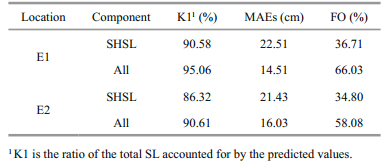
3.3 Prediction of total SLAs mentioned in Kurapov et al. (2017), the accurate prediction of the total SL required combining three main sources, including the sum of the tidal components, the SL affected by the sea level AP, and the ocean dynamic component (i.e., the low-frequency SL influenced by wind). As the two stations in this study, E1 and E2, were located in shallow embayment, the global tidal models did not provide an accurate estimate for tides (Shum et al., 1997; Wang et al., 2010). Therefore, the observed total SL was filtered using a cosine-lanczos filter with a low frequency cutoff of 0.8 cpd, and the high-pass result was taken as the first component, labelled as SHSL. The best predicted SLSL using the multivariable linear regression model was taken as the sum of the second component and the third component.
As shown in Figs. 2a and 3a, SLs in the high frequency bands were the significant contributor to the total SL. Therefore, the predicted SLs, only using SHSL, accounted for 90.58% and 86.32% of the total SLs at E1 and E2 (Table 5), respectively. However, the SLSLs were greater than 0.5 m at both E1 and E2 in some cases (Fig. 4a), so the predicted SLs only using SHSL, at both E1 and E2, were slightly far from the total SLs, as shown in Fig. 8a for E1 and Fig. 8b for E2.
|

|
| Fig.8 Time series of the observed total SL (grey line), the SHSL (black line), and the predicted total SL combining the SHSL and the SLSL predicted using the multivariable linear regression model (red line), at (a) E1 and (b) E2 |
When all of the three components were summed up to be the predicted SLs, the predicted SLs at both E1 and E2 were much closer to the total SL than those only using SHSL, as shown in Table 5. In detail, FOs were 66.03% and 58.08% at E1 and E2, which were improved as much as additional 29.32% and 23.28% compared to those only using SHSL, respectively. Similar to prediction of SLSLs at E1 and E2, the predicted SLs at E1 and E2 were slightly far from the total SLs near the local extrema (Fig. 8). In addition, the predicted SL at E1 was closer to the observed total SL than that at E2.
The aforementioned results indicated that the sum of the tidal components, i.e. SHSL, was the dominant source for predicting the total SL and the SL influenced by the atmospheric forcing cannot be neglected. When the SLSLs predicted using the multivariable linear regression model were considered, the predicted SLs could be significantly improved.
4 DISCUSSIONThe dominant wind orientations influencing SLSL are 65° at E1 and 55° at E2, respectively, which are nearly perpendicular to the southwest coastline of the Bohai Bay. The relationships between SLSLs and SWs at the corresponding orientations are negative (R=-0.47 at E1 and R=-0.32 at E2), indicating that the onshore winds will raise local SL and the offshore winds will reduce local SL. As E1 is close to the coastline, the SLSL is slightly larger; besides, the SLSL is more sensitive to the across-shore winds, as the corresponding regression coefficients, including α2, β1 and γ1, at E1 are much larger than those at E2. The aforementioned results show that the SLSLs in the Bohai Bay, which is a typical semi-enclosed coastal sea, are mostly influenced by the across-shore winds, which is not similar to that near the continental shelf (e.g., Hsueh and Romea, 1983; Zhao and Cao, 1987). Therefore, the predictions of the SLSLs in the local waters depend on different factors, which should be performed carefully at a special location.
The regression coefficients between SLSL and AP are negative, at both E1 and E2, which is the same as that in the IB formula. However, a 1-mb change in barometric pressure produces a 1.00×10⁻² m variation in sea level with sign inverted in the classic IB formula (Paraso and Valle-Levinson, 1996), while the corresponding variations in sea level are about 1.61×10⁻² m and 1.59×10⁻² m with sign inverted at E1 and E2, respectively, indicating the ocean response to AP is slightly far from a classical IB response.
The predicted SLSL and total SL at E1 are much closer to the observations than those at E2, indicating that the prediction of SLSL using the linear regression is much more effective for the shallow waters. The advection and other dynamic conditions make the prediction of SLSL in the deep and open waters like E2 be less accurate. When the total SL is predicted, the FOs are 66.03% and 58.08% at E1 and E2, respectively, which do not reach the target level (90%) in Kurapov et al. (2017), but FOs are improved with a reduction of 79.87% and 66.90% at E1 and E2 compared to those only using the sum of tidal components, respectively. It should be noted that if the much more accurate predictions are needed, the numerical simulation using the dynamical model with data assimilation is the most effective method, especially for these two observation stations located in a semi-enclosed coastal sea. As the tides and other high frequency bands account for the most part of the total SL, the accurate prediction for them is critical when the total SL is predicted. The simulation of tides using the traditional dynamical models is forced by the open boundary conditions retrieved from OTIS or other global tidal model, but these cannot provide an accurate estimate for tides in the shallow waters (Shum et al., 1997; Wang et al., 2010). Therefore, the data assimilation is necessary to be implemented (e.g., He et al., 2004; Zhang and Lu, 2010; Cao et al., 2012). In the future, a dynamical model with data assimilation will be developed to simulate the tides and the ocean dynamic component influenced by atmospheric forcing to further improve the prediction accuracy.
5 CONCLUSIONDuring the period from 19 August 2014 to 18 November 2014, the total SL, wind, and sea level AP were observed hourly at E1 and E2 stations in the Bohai Bay, China. As the Bohai Bay is a typical semienclosed coastal sea and has limited water exchange with the ocean (Meng et al., 2008), the SLSLs at E1 and E2 were almost the same as each other, but the winds were not.
The SLSLs at both E1 and E2 were influenced by the winds with similar maximum coherent condition and dominant wind orientation. At E1, SLSL was highly coherent with SW at 50° at about 0.375 cpd; similarly, SLSL at E2 was highly coherent with SW at 30° at about 0.375 cpd. Overall, SLSLs were dominantly influenced by SW at 65° for E1 and at 55° for E2, respectively.
The linear regression was taken as the simple prediction method. The predicted SLSL, using the multivariable linear regression model of wind component at dominant orientation and AP, was much closer to the observed values than that predicted using only wind component or using the combination of the linear regression model of wind component at dominant orientation and IB, at both E1 and E2. When the best predicted SLSLs were taken as a part of the predicted total SL, the MAEs between the predicted and observed total SLs were 14.51 cm at E1 and 16.03 cm at E2, respectively; moreover, FOs were 66.03% at E1 and 58.08% at E2, which were improved by 79.87% and 66.90% compared to those only using the sum of tidal components, respectively. The prediction results indicated that the simple prediction method was effective for the shallow waters near coast, like E1 and E2, which can obtain better results than the traditional method. For the prediction of the SL variability in the coastal shallow waters, the SLSL influenced by atmospheric forcing can be simply predicted using the linear regression relationship between SLSL and atmospheric forcing, including SW at dominant wind orientation and AP; besides, neither wind nor AP can be ignored.
6 DATA AVAILABILITY STATEMENTThe datasets analyzed during the current study are available from the corresponding author on reasonable request.
7 ACKNOWLEDGEMENTThe authors would like to thank the two anonymous reviewers for the constructive suggestions to greatly improve the manuscript. Thanks are extended to Carlos Adrian Vargas Aguilera (nubeobscura@ hotmail.com) for sharing the matlab code of lanczos filter.
Andres M, Gawarkiewicz G G, Toole J M. 2013. Interannual sea level variability in the western North Atlantic:regional forcing and remote response. Geophysical Research Letters, 40(22): 5915-5919.
DOI:10.1002/2013GL058013 |
Cao A Z, Guo Z, Lü X Q. 2012. Inversion of two-dimensional tidal open boundary conditions of M2 constituent in the Bohai and Yellow Seas. Chinese Journal of Oceanology and Limnology, 30(5): 868-875.
DOI:10.1007/s00343-012-1185-9 |
Carrere L, Faugère Y, Ablain M. 2016. Major improvement of altimetry sea level estimations using pressure-derived corrections based on ERA-Interim atmospheric reanalysis. Ocean Science, 12(3): 825-842.
DOI:10.5194/os-12-825-2016 |
Carrère L, Lyard F. 2003. Modeling the barotropic response of the global ocean to atmospheric wind and pressure forcing-comparisons with observations. Geophysical Research Letters, 30(6): 1275.
|
Castro B M, Lee T N. 1995. Wind-forced sea level variability on the southeast Brazilian shelf. Journal of Geophysical Research:Oceans, 100(C8): 16045-16056.
DOI:10.1029/95jc01499 |
Chen X Y, Zhang X B, Church J A, Watson C S, King M A, Monselesan D, Legresy B, Harig C. 2017. The increasing rate of global mean sea-level rise during 1993-2014. Nature Climate Change, 7(7): 492-497.
DOI:10.1038/nclimate3325 |
Cheng Y C, Andersen O B. 2011. Multimission empirical ocean tide modeling for shallow waters and polar seas. Journal of Geophysical Research:Oceans, 116(C11): C11001.
DOI:10.1029/2011jc007172 |
Egbert G D, Erofeeva S Y. 2002. Efficient inverse modeling of barotropic ocean tides. Journal of Atmospheric and Oceanic Technology, 19(2): 183-204.
DOI:10.1175/1520-0426(2002)019<0183:eimobo>2.0.co;2 |
Garrett C. 2001. What is the "near-inertial" band and why is it different from the rest of the internal wave spectrum?. Journal of Physical Oceanography, 31(4): 962-971.
DOI:10.1175/1520-0485(2001)031<0962:witnib>2.0.co;2 |
Grinsted A, Moore J C, Jevrejeva S. 2004. Application of the cross wavelet transform and wavelet coherence to geophysical time series. Nonlinear Processes in Geophysics, 11(5-6): 561-566.
DOI:10.5194/npg-11-561-2004 |
He Y J, Lu X Q, Qiu Z F, Zhao J P. 2004. Shallow water tidal constituents in the Bohai Sea and the Yellow Sea from a numerical adjoint model with TOPEX/POSEIDON altimeter data. Continental Shelf Research, 24(13-14): 1521-1529.
DOI:10.1016/j.csr.2004.05.008 |
Hsueh Y, Romea R D. 1983. Wintertime winds and coastal sealevel fluctuations in the northeast China Sea. Part I:observations. Journal of Physical Oceanography, 13(11): 2091-2106.
DOI:10.1175/1520-0485(1983)013<2091:wwacsl>2.0.co;2 |
Kurapov A L, Erofeeva S Y, Myers E. 2017. Coastal sea level variability in the US West Coast Ocean Forecast System(WCOFS). Ocean Dynamics, 67(1): 23-36.
DOI:10.1007/s10236-016-1013-4 |
Le Provost C, Lyard F, Molines J M, Genco M L, Rabilloud F. 1998. A hydrodynamic ocean tide model improved by assimilating a satellite altimeter-derived data set. Journal of Geophysical Research:Oceans, 103(C3): 5513-5529.
DOI:10.1029/97jc01733 |
Li K P, Yang K Q. 1983. The non-periodic sea level variation in relation to wind and pressure at the Bohai Bay. Marine Sciences, (2): 12-15.
(in Chinese with English abstract) |
Liu K X, Wang H, Fu S J, Gao Z G, Dong J X, Feng J L, Gao T. 2017. Evaluation of sea level rise in Bohai Bay and associated responses. Advances in Climate Change Research, 8(1): 48-56.
DOI:10.1016/j.accre.2017.03.006 |
Matsumoto K, Takanezawa T, Ooe M. 2000. Ocean tide models developed by assimilating TOPEX/POSEIDON altimeter data into hydrodynamical model:a global model and a regional model around Japan. Journal of Oceanography, 56(5): 567-581.
DOI:10.1023/A:1011157212596 |
Mellor G L, Ezer T. 1995. Sea level variations induced by heating and cooling:an evaluation of the Boussinesq approximation in ocean models. Journal of Geophysical Research:Oceans, 100(C10): 20565-20577.
DOI:10.1029/95jc02442 |
Meng W, Qin Y W, Zheng B H, Zhang L. 2008. Heavy metal pollution in Tianjin Bohai bay, China. Journal of Environmental Sciences, 20(7): 814-819.
DOI:10.1016/s1001-0742(08)62131-2 |
Paraso M C, Valle-Levinson A. 1996. Meteorological influences on sea level and water temperature in the lower Chesapeake bay:1992. Estuaries, 19(3): 548-561.
DOI:10.2307/1352517 |
Piecuch C G, Dangendorf S, Ponte R M, Marcos M. 2016. Annual sea level changes on the North American Northeast Coast:influence of local winds and barotropic motions. Journal of Climate, 29(13): 4801-4816.
DOI:10.1175/jcli-d-16-0048.1 |
Quartly G D, Legeais J F, Ablain M, Zawadzki L, Fernandes M J, Rudenko S, Carrère L, García P N, Cipollini P, Andersen O B, Poisson J C, Njiche S M, Cazenave A, Benveniste J. 2017. A new phase in the production of quality-controlled sea level data. Earth System Science Data, 9(2): 557-572.
DOI:10.5194/essd-9-557-2017 |
Sandstrom H. 1980. On the wind-induced sea level changes on the Scotian shelf. Journal of Geophysical Research:Oceans, 85(C1): 461-468.
DOI:10.1029/jc085ic01p00461 |
Shum C K, Woodworth P L, Andersen O B, Egbert G D, Francis O, King C, Klosko S M, Le Provost C, Li X, Molines J M, Parke M E, Ray R D, Schlax M G, Stammer D, Tierney C C, Vincent P, Wunsch C I. 1997. Accuracy assessment of recent ocean tide models. Journal of Geophysical Research:Oceans, 102(C11): 25173-25194.
DOI:10.1029/97jc00445 |
Sun P, Yu G, Chen Z Z, Hu J Y, Liu G X, Xu D H. 2015. Diagnostic model construction and example analysis of habitat degradation in enclosed bay:Ⅲ. Sansha Bay habitat restoration strategy. Chinese Journal of Oceanology and Limnology, 33(2): 477-489.
DOI:10.1007/s00343-015-4169-8 |
Thompson P R, Merrifield M A, Wells J R, Chang C M. 2014. Wind-driven coastal sea level variability in the northeast pacific. Journal of Climate, 27(12): 4733-4751.
DOI:10.1175/jcli-d-13-00225.1 |
Wang Y H, Fang G H, Wei Z X, Wang Y G, Wang X Y. 2010. Accuracy assessment of global ocean tide models base on satellite altimetry. Advances in Earth Science, 25(4): 353-359.
(in Chinese with English abstract) |
Xu Z H, Yin B S, Hou Y J, Xu Y S. 2013. Variability of internal tides and near-inertial waves on the continental slope of the northwestern South China Sea. Journal of Geophysical Research:Oceans, 118(1): 197-211.
DOI:10.1029/2012jc008212 |
Zhang A J, Hess K W, Wei E, Myers E. 2006. Implementation of Model Skill Assessment Software for Water Level and Current in Tidal Regions. NOAA Technical Report NOS CS 24. NOAA, Silver Spring, MD. (2006-03). https://repository.library.noaa.gov/view/noaa/2204. Accessed on 2018-6-21.
|
Zhang J C, Lu X Q. 2010. Inversion of three-dimensional tidal currents in marginal seas by assimilating satellite altimetry. Computer Methods in Applied Mechanics and Engineering, 199(49-52): 3125-3136.
DOI:10.1016/j.cma.2010.06.014 |
Zhao B R, Cao D M. 1987. Wintertime low frequency fluctuations of Chinese coastal sea-level in the Huanghai Sea and the East China Sea. Oceanologia et Limnologia Sinica, 18(6): 563-574.
(in Chinese with English abstract) |