 2019, Vol. 37
Institute of Oceanology, Chinese Academy of Sciences
Article Information
- ZHAO Yili, LI Huimin, CHEN Chuntao, ZHU Jianhua
- Verification and recalibration of HY-2A microwave radiometer brightness temperature
- Journal of Oceanology and Limnology, 37(3): 968-981
- http://dx.doi.org/10.1007/s00343-019-8073-5
Article History
- Received Apr. 3, 2018
- accepted in principle Jul. 23, 2018
- accepted for publication Aug. 15, 2018


2 Laboratoire d'Oceanographie Physique et Spatiale, Ifremer, Plouzané 29280, France
Satellite-based microwave radiometers (RMs) play an important role in the Earth observation. The measurements of microwave RMs are applied operationally in numerical prediction systems, global climate change monitoring, and many oceanographic studies (Bell et al., 2008; Rozoff et al., 2015).
To measure ocean dynamic environmental parameters, China launched HY-2A on 16 August 2011, the first one of the HY-2 satellite series. Four microwave instruments were deployed onboard HY- 2A, i.e., a microwave scatterometer, radar altimeter, scanning microwave RM, and another microwave RM used for altimeter calibration. HY-2A operated in a 99.3° inclined sun-synchronous orbit at 970-km altitude and the local time of the ascending node was 6:00 pm (Jiang et al., 2012). The designed life of HY- 2A was just three years and after the designed life had finished, the orbit was changed in March 2016 to facilitate other scientific objectives.
The environmental products of the HY-2A RM were validated by (Huang et al., 2014a, b; Zhao et all., 2014; Guan and Liu, 2015; Liu et al., 2017) using in situ measurements and environmental products from other microwave RMs. For example, Zhao et all. (2014) evaluated RM sea surface temperature (SST) against buoy measurements and their derived results presented a root mean square error (RMSE) of about 1.7℃. Similarly, Liu et al. (2017) validated RM SST against WindSat SST and buoy measurements obtained during the period January 2012 to December 2014 and they also found the total RMSE was 1.7℃. Error analyses presented by Guan et al. (2015) showed the RMSE of RM SST on descending passes was less than on ascending passes. For RM sea surface wind speed (SSWS), Huang et al. (2014a) compared RM SSWS with WindSat SSWS and buoy observations and they obtained an RMSE of 1.9 m/s. An RMSE of RM columnar water vapor (WV) of 1.2 mm was reported by Huang et al. (2014b), based on comparison with special sensor microwave imager observations.
Brightness temperature (TB) is used to retrieve environmental parameters; however, only a few studies have been performed to evaluate its quality. Specifically, Li et al. (2014) and Wang et al. (2014) reported the cold calibration targets of the HY-2A RM are contaminated by radiation from the Earth because of the spillover of the cold mirror. This study focused on the HY-2 RM level 1B TB. The objective was to verify the accuracy of the HY-2A RM level 1B TB and to analyze the temporal variation of error. Furthermore, following analysis of the error sources, testing of RM TB recalibration was performed.
The characteristics of the HY-2A RM and HY-2A RM TB sensors, the auxiliary data, and the method used for verification are introduced in Sections 2, 3, and 4, respectively. The verification of the HY-2A RM TB and recalibration testing are introduced in Sections 5 and 6. Finally, a discussion and our conclusions are given in Sections 7 and 8, respectively.
2 SENSOR CHARACTERISTICSThe HY-2A RM was developed by the Chinese Academy of Space Technology (Xi'an) to detect SST, SSWS, atmospheric water vapor, and cloud liquid water content. The HY-2A RM was designed to work in five discrete bands (Table 1). The channels at 6.6 and 10.7 GHz share a two-frequency feed horn, whereas the others share a three-frequency feed horn (Jiang et al., 2012).

HY-2A RM uses a 1.2-m-diameter offset parabolic reflector to collect microwave radiation. The reflector is fixed at a 40° half-cone angle, which results in an Earth incidence angle of 47.7°. The instrument rotates continuously about an axis parallel to HY-2A with a period of 3.79 s. The scanning azimuth angle is about ±70° relative to the sub-satellite track, resulting in a 1 600-km-wide swath on the Earth's surface. As with most satellite-borne microwave RMs, HY-2A RM uses a stationary hot load of about 290 K and a cold mirror to provide primary calibration references for in-orbit calibration.
3 DATASET 3.1 RM level 1B brightness temperatureThe product of the HY-2A RM level 1B TB is produced by the National Satellite Oceanic Application Service of the State Oceanic Administration, China. According to the product definition, level 1B TB was generated from the level 1A product. The content of the level 1B product is divided into four groups depending on spatial resolution: one group saved TB in the original spatial resolution of each band, while the other three groups were resampled at the spatial resolution of the 6.6, 10.7, and 18.7 GHz channels (User's Guide available at http://www.nsoas.org.cn/NSOAS_En/Services/index.html). The TB in the original resolution was used in this study.
A set of TB images is shown in Fig. 1 as an example. The abnormally high values of TB at 6.6 and 10.7 GHz along the coastline are caused by the footprint size of the channels at these frequencies. In the preprocessing of level 1B TB, we excluded pixels over land and within 100 km of the coastline. Moreover, the polarization ratio p, defined in Eq.1, was employed to exclude TB polluted by land or ice:

|
| Fig.1 HY-2A RM TB images of the China Sea observed on 7 January 2012 |
 (1)
(1)where TB, V and TB, H indicate vertical and horizontal polarization, respectively (Brucker et al., 2014). In our study, p was calculated using TB at 6.6 GHz. We found most TBs with values of P < 0.21 were contaminated by land or ice and thus they were excluded. The filter created using TB at 6.6 GHz was applied to the channels at other frequencies.
3.2 Auxiliary dataThe auxiliary data used in this study comprised the WindSat environmental product version 7.0.1, produced by the Remote Sensing System (RSS). WindSat is the first fully polarimetric microwave RM, which was launched on 6 January 2003 aboard the Coriolis satellite (Gaiser et al., 2004). The RSS provides a suite of WindSat products, i.e., daily, threeday periods, weekly, and monthly. The daily product used in our study contained SST, SSWS, sea surface wind direction (SSWD), WV, columnar cloud liquid water (CL) and rain rate (RR). All parameters were mapped onto two global 0.25°×0.25° grids depending on ascending and descending passes.
The quality of the RSS WindSat products have been examined and validated in many previous studies (Meissner and Wentz, 2005; Zhao et al., 2014; Wentz, 2015; Zhang et al., 2016; Liu et al., 2017). For example, WindSat retrieval of SST, SSWS, WV, and CL has been validated with accuracy of 0.83 K, 0.81 m/s, 0.73 mm, and 0.025 mm, respectively (Meissner and Wentz, 2005). For SSWD, the standard deviation (SD), with reference to the National Centers for Environmental Prediction Global Data Assimilation System, was found < 20°, while that for SSWS was found >8 m/s. Zhao et al. (2014) validated the RSS WindSat SST between 1 January 2012 and 30 June 2012 versus buoy measurements and their results indicated an RMSE of about 0.6 K. The RMSE of WindSat SSWS, with reference to in situ measurements during the same period, was verified as 1.17 m/s (Liu et al., 2017). For long-term RSS WindSat product validation, Zhang et al. (2016) compared WindSat SST and SSWS with buoy data obtained during 2004–2013, and the total RMSE of SST and SSWS was less than 0.7 K and 1.2 m/s, respectively. Furthermore, no temporal trend was shown in the results. Wentz (2015) compared the environmental parameters of WindSat products with those observed by the Tropical Rainfall Measuring Mission Microwave Imager (TMI) during 2003– 2015, and the time series of the differences was established as stable during this period.
The validation results mentioned above suggest the RSS WindSat products have good accuracy and stability and thus, they could be used in our study with confidence.
3.3 Collocation of RM and WindSat dataWe collected global HY-2A RM level 1B TB products and RSS WindSat products from 1 January 2012 to 31 July 2015. To perform accurate verification and recalibration testing, we collocated the RM TB with WindSat environmental parameters via the following steps. For spatial collocation, the distance between locations of RMTBand WindSat measurement was constrained to < 25 km. The time difference between RM measurement and WindSat sensing was also constrained to < 60 min. Furthermore, RM TB with WindSat RR>0 mm/h and CL>0.18 mm were excluded to avoid rain contamination. The total number of collocations was 53 768 589.
In the collocation, WindSat products (i.e., SST, SSWS, SSWD, WV, and CL) were used as inputs for the ocean-atmosphere radiative transfer model (RTM) to simulate TB at the top of the atmosphere. The TB simulated by the RTM was used as reference against which to verify the quality of HY-2A and for the development of the recalibration algorithm.
4 METHODOLOGYIn our study, only the HY-2A RM level 1B TBs observed over the global ocean were considered. The TB simulated by the RTM was used as reference for verification and recalibration of the HY-2A RM level 1B TB. Several RTMs were used for post-launch calibration of the satellite-based microwave RM (Kroodsma et al., 2012; Alsweiss et al., 2015; Draper et all., 2015; Wentz and Draper, 2016). Draper et all. (2015) used an RTM developed by the RSS to calibrate the Global Precipitation Measurement Microwave Imager (GMI). They found a difference between the GMI measurement and the RTM simulation of < 0.8 K for all channels. Another report by Wentz and Draper (2016) indicated the RSS RTM could simulate GMI TB with an RMSE of < 0.25 K for all channels.
For the RTM employed in this study, we used a combination of the latest revised RSS ocean surface emission model presented by Meissner and Wentz (2012) and an atmospheric RTM (ARTM) presented by Bettenhausen et al. (2006). The ocean surface emission model covers frequencies of 6–90 GHz and incidence angles of 0°–65°. The ARTM was developed for WindSat, which operates at five working frequencies: 6.8, 10.7, 18.7, 23.8, and 37.0 GHz. At these frequencies, the atmospheric contribution is primarily dependent on WV and CL rather than on the detailed shape of the vertical profiles (Wentz, 1997); hence, the ARTM was designed to use WV and CL as inputs. It should be noted that we neglected the difference between the lowest ARTM frequency (i.e., 6.8 GHz) and the lowest HY-2 RM frequency (i.e., 6.6 GHz) because the atmosphere is almost transparent and the attenuation and radiation are stable in this microwave band (Liebe, 1989). The RTM could be expressed as:
 (2)
(2) (3)
(3) (4)
(4)where TB represents sea surface direct emission, TBD is atmospheric downwelling radiation, and TB, scat is atmospheric path length correction. TS is SST. Subscript p indicates vertical polarization (V) or horizontal polarization (H). E is the emission coefficient of the sea surface, whereas R is the sea surface reflection coefficient, which could be calculated by R=1–E. E is a function of SST, SSWS, SSWD, and sea surface salinity (SSS). TBΩ is the downwelling sky radiation scattered from the ocean. Ωp was calculated using the surface GO model (Meissner and Wentz, 2012). Atmospheric transmission, upwelling, and downwelling TBs are represented by τ, TBU, and TBD, respectively. These three parameters could be computed with WV and CL. Tcold is an effective cold space temperature accounting for the deviation of the Rayleigh-Jeans approximation from Planck's law, which is given in Table 26 of Meissner et al. (2012). To simulate the TB at the RM measuring location and time, the collocated WindSat environmental products (i.e., SST, SSWS, SSWD, WV, and CL) were used as RTM inputs. For SSS, we used a constant value of 35.5.
Here, we analyze the accuracy and stability of the RM TB using both statistical and graphical methods. Statistical indices including bias and SD are employed to analyze the difference between the RM TB and that simulated by the RTM. These two parameters are defined as follows:
 (5)
(5)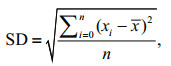 (6)
(6)where TB, RM and TB, RTM represent the TB measured by the RM and simulated by the RTM, respectively, xi=TB, RM, i–TB, RTM, i, and is the mean of x.
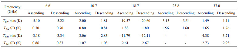
5 VERIFICATION 5.1 Comparison of HY-2A RM TB and the RTM simulationFor verification, we first compared all the collocations of TB measured by the RM and simulated by the RTM. Figure 2 shows density plots of RM TB (y-axis) against RTM simulations (x-axis) for nine channels. The total bias and SD of the RM TB, with reference to the RTM simulation, are estimated based on Eqs.5 and 6. Table 2 presents the biases and SDs in the nine channels of the RM. The SDs are found to have frequency dependence. The biases and SDs of the ascending and descending passes are slightly different. Moreover, the biases at 6.6, 18.7, and 23.8 GHz are negative, indicating the RM measurements at these frequencies are underestimations. Conversely, the RM measurements at 10.7 and 37.0 GHz are overestimations. The biases at 18.7 GHz, particularly the bias of the vertically polarized TB, suggest the HY-2A RM has calibration problems at this frequency.

|
| Fig.2 Density plots of TB measured by the RM against TB simulated by the RTM in nine channels of the HY-2A RM |
The total bias and SD indicate the general quality of the RM level 1B TB. To verify the quality and stability of the RM level 1B TB in detail, we performed further analyses. First, we subtracted the total bias (values in Table 2) from the RM TB and we recalculated the difference between the RM TB and the RTM simulation. Then, the new daily differences were averaged with latitude bins of 0.25° to obtain the residual bias. The same processing was performed for each day from 1 January 2012 to 31 July 2015 to examine the stability of the residual bias at the same latitude.
Figures 3 and 4 illustrate the change of the residual bias with latitude and measurement date for ascending and descending passes, respectively. All the subplots in these two figures show obvious seasonal variation. The residual bias of the ascending passes at 6.6 and 10.7 GHz in January in the Southern Hemisphere is less than in the Northern Hemisphere. This trend changes with the date, in that the residual bias in the Northern Hemisphere decreases, while it increases in the Southern Hemisphere; however, the trend is totally reversed in July. In contrast to the variation at high latitudes, the residual bias near the equator has weak seasonal variation. In addition, the residual bias of the ascending passes can be seen to be abnormally high near latitudes of about 30°N. According to Wentz (2015), this abnormal phenomenon at fixed locations could be caused by broadcasts from geostationary satellites entering the cold mirror. Similar to the temporal variation of the residual bias at 6.6 and 10 GHz, that at 18.7, 23.8, and 37.0 GHz also shows seasonal variation but with intensified amplitude. The values of residual bias near the equator shown in all the plots in Figs. 3 and 4 are almost constant during the analysis period. Compared with the variation of the residual bias of the descending passes, that of the ascending passes in the Southern Hemisphere is relatively weak.

|
| Fig.3 Change of residual bias with latitude and measurement date from 1 January 2012 to 31 July 2015 for ascending passes |

|
| Fig.4 Change of residual bias with latitude and measurement date from 1 January 2012 to 31 July 2015 for descending passes |
Comparison of the HY-2A RM level 1B TB and the RTM simulation reveals significant bias and obvious seasonal variation. Even though the SD of every HY- 2A RM channel appears reasonable, it is worse than that of the GMI, which has a better calibration system. We compare the in-orbit calibration of the HY-2A RM and GMI in Section 7.
5.2 Error analysis of HY-2A RM TBPrevious studies by Wentz (2015) and Kunkee et all. (2008) suggested the errors of satellite-borne microwave RM measurements could be attributable to several factors such as antenna spillover, the reflectivity and emissivity of the main reflector, and receiver nonlinearity. Several of these potential error sources could be measured before launch but they represent significant uncertainty for satellites in orbit (Kunkee et al., 2008). The major challenge is the prelaunch determination of the antenna spillover coefficients because it requires accurate knowledge of antenna patterns over the entire back lobes of the main reflector (Wentz and Draper, 2016). By definition, the antenna temperature measured by a microwave RM is the TB of the surrounding environment integrated over the gain pattern of the sensor. It could be expressed as:
 (7)
(7)where η is the antenna spillover coefficient, and TB, earth and TB, space are TB of the Earth target alnd cold space, respectively (Wentz, 2015). The analysis by Wentz (2013) indicated that most satellite microwave RMs have a η error of about 1%, which translates into an error of about 2 K in TB, Earth. The spillover coefficients of the HY-2A RM, estimated based on prelaunch measurements, are 0.078, 0.028, 0.151, 0.06, and 0.037 for the 6.6, 10.7, 18.7, 23.8, and 37-GHz channels, respectively.
In addition to antenna spillover, the emissivity of the main reflector also contributes to the bias of the HY-2A RM TB. The HY-2A RM uses an emissive main reflector, i.e., the TB received by the feed horn comprises the TB reflected by the main reflector and the radiation that comes from the main reflector itself. Considering the effects of reflectivity and emissivity of the main reflector, Eq.7 can be rewritten as:
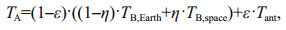 (8)
(8)where ε and Tant are the emissivity and physical temperature of the main reflector, respectively Wentz, (2015). The value of ε of the TMI antenna was reported by Wentz (2015) to range from 0.025 to 0.049 and to have spectral dependency. The Tant of the TMI, as estimated by Wentz (2015), ranges from 265 to 315 K, which could introduce an absolute bias of about 0.3– 1.3 K to TA. The HY-2A RM Tant, measured by three thermistors attached to the antenna, ranges from 290 to 400 K (see Fig. 5). The larger variation of the HY- 2A RM Tant increases the contribution of antenna emission to the bias of RM TB.

|
| Fig.5 The HY-2A RM antenna physical temperature (Tant) variation (one year: 2012) with latitude and measurement date from 1 January a. Tant of ascending passes; b. Tant of descending passes. |
By transforming Eq.8, we could calculate the difference between the antenna temperature and the TB of the Earth target by:
 (9)
(9)The first term on the right-hand side is the contribution of the antenna spillover coefficient. The cold space TB has an approximation of 2.73 K, which is lower than the TB of the Earth target. This means that the antenna spillover coefficient contributes negative bias to TA. The second term on the right-hand side indicates the bias induced by physical emission of the antenna. Usually, the physical temperature of the antenna is warmer than 260 K, which results in positive bias. The total bias on the left-hand side is the sum of these two contributions, which means it is difficult to separate them precisely. Wentz (2015) used a rainforest as a target to estimate the antenna spillover coefficients because the TB of a rainforest is about 275 K, which is close to the mean physical temperature of the TMI antenna (290 K). In a oneyear period, the Tant of the HY-2A RM over the Amazon rainforest ranged from 293 to 336 K for ascending passes and it ranged from 311 to 340 K for descending passes, which means the method of Wentz (2015)) does not work for the HY-2A RM. The worse condition is a maximum of RM Tant of around 400 K (see Fig. 5) because the shape of the antenna would vary at this temperature, resulting in the spillover coefficients changing.
The third factor concerns the uncertainty attributable to calibration targets, which is a common problem for most satellite-borne microwave RMs. The HY-2A RM uses a hot load and a cold mirror to provide references to convert the count to antenna temperature. Assuming the HY-2A RM has true linear response to TA, the conversion could be expressed by:
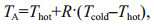 (10)
(10)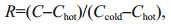 (11)
(11)where TA is the antenna temperature, Thot is the hot load physical temperature, and Tcold is the cold space TB. Here, C, Chot, and Ccold are the counts of the sensor when it views the Earth, hot load, and cold mirror, respectively (Wentz, 2015). The conversion coefficient R depends on frequency and polarization. Because of solar intrusions, the thermal distribution of the hot load becomes irregular and that makes the thermistor measurements (Thot) fail to present the real temperature, resulting in an error in the TA calculation (Wentz and Draper, 2016). Another problem of the HY-2 RM inorbit calibration is that a small amount of TB from the Earth is reflected directly into the feed horn because of the spillover of the cold mirror. Even if a correction was performed to reduce the contamination of Tcold, it would introduce considerable uncertainty to the RM level 1B TB (Li et al., 2014). Aside from the antenna spillover, antenna physical emission, and uncertainty of calibration targets, the HY-2A RM also suffers other sources of error, e.g., cross-polarization coupling, beam pointing, frequency stability, and pass band response.
6 RECALIBRATION 6.1 Recalibration algorithmConsidering all the error sources of the HY-2A RM, the TB of the Earth target could be estimated by combining Eqs. 7–10:
 (12)
(12)where δ indicates the errors caused by error sources other than the antenna spillover and antenna physical emission. For training the recalibration algorithm, the TB, RTM is used as TB, Earth. As discussed in Section 5.2, it is difficult to estimate ε and real values of η for HY- 2A; specifically, the value of η for the HY-2A RM changes with Tant, which means all four terms on the right-hand side are a function of Tant. Moreover, information regarding the errors of calibration targets is not contained in the datasets. Thus, it is not supported to segment the errors from different error sources and to perform precise recalibration based on Eq.12.
Because of the lack of error source segmentation, we designed a recalibration testing using a statistical method. In the recalibration, TB, space is approximated to a constant of 2.73 K and δ is assumed isolated from TA and Tant. First, we treat TB, Earth as a function of TA and Tant. Then, the calibrated TB, RM at the first step (TB0) could be expressed by:
 (13)
(13)where the coefficients C0 and C1 are estimated based on linear regression. In the linear regression, TB, RTM is used as TB0. To avoid the effect of Tant, we only use collocations with Tant=325 K in this step. Table 3 presents the values of C0 and C1 for all the channels of the HY-2A RM.
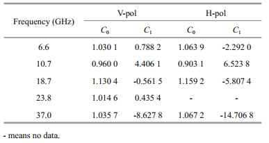
In the second step, the contribution of Tant to the residual differences between TB0 and TB, RTM are analyzed against Tant based on the assumption that C0 is independent of Tant:
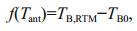 (14)
(14)where f(Tant) represents the variation of the residual differences with reference to Tant. Then, the calibrated TB, RM at the second step (TB1) could be expressed as:
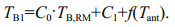 (15)
(15)As shown by Fig. 6, the amplitudes of f(Tant) increase with increasing frequency. Moreover, sharp variations of f(Tant) appear at around Tant=341 K for all channels. Checking with the third term on the right-hand side of Eq.12, the variation of f(Tant) confirms the spillover coefficient (η) changes with Tant. This is because antenna emissivity ε is determined by the material and surface of the antenna, which is independent of Tant. In the recalibration testing, we use lookup tables of f(Tant), which can maintain the continuity around Tant=341 K. In addition, we also notice a sharp increase of the SD at around 320 K in several channels, especially 23.8 GHz V-pol. A possible reason for this is that the variation of the spillover coefficients around 320 K is not smooth. This could be verified by the small fluctuation at around 320 K shown by the bias.

|
| Fig.6 Change of f(Tant) with antenna physical temperature in nine HY-2A RM channels Black line represents f(Tant) and gray dashed line represents 1−SD of TB0. |
Finally, the residual difference between TB1 and TB, RTM could be calculated as follows:
 (16)
(16)where Δ contains the contribution of the uncertainty of the calibration targets (ΔThot and ΔTcold) due to solar intrusion and contamination from the Earth. The variations of ΔThot and ΔTcold change with latitude, pass direction, and date. We constructed lookup tables of Δ to refer to latitude and days from the first day of the year (1 January) for the ascending and descending passes. Figure 7 shows an example of the Δ lookup table for the 37.0-GHz horizontal polarization channel. It shows the values of Δ for the 37.0-GHz horizontal polarization channel are negative in the Northern Hemisphere during April–July for both ascending and descending passes with slight differences. Most of the values of Δ are positive in the Southern Hemisphere. The feature shown in Fig. 7a between 70°S and 46°S in June is similar to that shown by the Tant image (Fig. 5a). The most probable reason for this is strong sunshine in this area and the period that caused Tant to be high and solar intrusion to be strong.

|
| Fig.7 Lookup tables of Δ for 37.0-GHz horizontal polarization channel a. ascending passes; b. descending passes |
After the three-step training, the recalibration algorithm could be expressed as:
 (17)
(17)where TB, cal is the recalibrated HY-2A RM level 1B TB. The first two terms on the right-hand side primarily calibrate the bias contributed by antenna spillover and antenna physical emission. The third term was added to remove the effect caused by variation of the antenna physical temperature. The final term eliminates the seasonal bias due to solar intrusion and contamination from the Earth.
6.2 Recalibration validationWe used the collocations between 1 January and 31 December 2012 to estimate C0 and C1 of Eq.13 and to create lookup tables of f(Tant) and Δ in Eq.14. Then, we performed recalibration of the HY-2A RM level 1B TB from 1 January 2013 to 31 July 2015 and evaluated the recalibrated results using the same method as described in Section 4.
The total errors of the recalibrated HY-2A RM TB are given in Table 4. Compared with the errors given in Table 2, the absolute bias of the recalibrated TB, with reference to the RTM simulation, is reduced to < 0.4 K for all channels, while the SD is also diminished. The residual bias of the calibrated RM TB is shown in Figs. 8 and 9. The seasonal variation shown in Figs. 3 and 4 has vanished in Figs. 8 and 9.


|
| Fig.8 Residual bias of recalibrated HY-2A RM level 1B TB variation with latitude and day from 1 January 2013 to 31 July 2015 over ascending passes |

|
| Fig.9 Residual bias of recalibrated HY-2A RM level 1B TB variation with latitude and day from 1 January 2013 to 31 July 2015 over descending passes |
The evaluation results confirm the feasibility of our HY-2A RM recalibration. The recalibration algorithm described in Section 6.1 could be used to calibrate the errors caused by antenna spillover, antenna physical emission, and other error sources that have seasonal variation. However, for errors with short-term variation, e.g., those induced by spacecraft rolling, sensor pointing will require further calibration.
7 DISCUSSIONThe empirical recalibration algorithm presented in this paper was designed for the HY-2A & B RM level 1B TB product. It represents an optimal solution for the satellite-based RM for which it is difficult to segment the error sources of the measurement. If the RM (e.g., GMI) could provide sufficient information to analyze the contribution of each error source, the method presented by Wentz and Draper (2016) would be a better solution.
Compared with the GMI, which marks a milestone of satellite microwave radiometry, the in-orbit calibration methods, material of the main reflector, stabilities of the cold and hot calibration targets, and other sensor characteristics constrain the accuracy of the HY-2A RM TB products. The TB RMSE of all GMI channels that refer to the RTM simulation are < 0.25 K, i.e., much better than those of the HY-2A RM TB after recalibration (Draper et al., 2015; Wentz and Draper, 2016).
The GMI employs a non-emissivity antenna that makes it free of antenna physical emission. The most important improvement of in-orbit calibration is the cold space calibration, which provides a means for direct computation of the spillover coefficients rather than relying on estimations based on prelaunch measurements. Accurate spillover coefficients could improve the accuracy of absolute calibration substantially. In addition, benefitting from noise diodes, which measure RM nonlinearity, calibration accuracies could be maintained from 80–300 K (Wentz and Draper, 2016). The GMI provides suggestions for the improvement of microwave RMs onboard future satellites of the HY-2 series.
8 CONCLUSIONWe verified the HY-2A RM level 1B TB using a simulation of an ocean-atmosphere RTM as a reference. The verification results that included the total bias, total SD, and time-varying analyses suggested the HY-2A RM has problems concerning TB calibration. Because of spillover and the physical emissivity of the main antenna, spillover of the cold mirror, and solar intrusion, the RM level 1B TB suffers many sources of error.
To improve the quality of HY-2A RM level 1B TB products, we performed recalibration testing. As the high physical temperature of the RM main antenna increases the error merging, quantitative error segregation is impossible. Based on error analyses and several assumptions, a statistical algorithm was designed for the recalibration of the RM level 1B TB. Collocation data from 2012 were used to train the recalibration algorithm, which was applied to calibrate the RM level 1B TB from 1 January 2013 to 31 July 2015. Compared with the RM TB before recalibration, our statistical algorithm could calibrate the bias of the RM channels well, eliminating seasonal variation and reducing the SD. The recalibration performed in this study could improve the quality of the HY-2A RM and it could also be helpful for the calibration of the similar scanning microwave RM onboard HY-2B, which is planned for launched in 2018.
9 DATA AVAILABILITY STATEMENTThe HY-2A RM level 1B data are available from the National Satellite Ocean Application Service (NSOAS) but restrictions apply to the availability of these data, which were used under license for the current study and so are not publicly available. Data are however available from the authors upon reasonable request and with the permission of NSOAS. WindSat data are produced by Remote Sensing Systems (RSS) and sponsored by the NASA Earth Science MEaSUREs DISCOVER Project and the NASA Earth Science Physical Oceanography Program. The RSS WindSat data are available at ftp://ftp.ssmi.com/windsat.
10 ACKNOWLEDGMENTThe authors would like to thank the Remote Sensing System for supporting the WindSat environmental products and RTM. We also acknowledge JIN Xu from the China Academy of Space Technology (Xi'an) for helpful discussion on the characteristics of the HY-2A scanning microwave radiometer. The author Yili ZHAO thank the China Scholarship Council for supporting this study at LOPS/IFREMER in France.
Alsweiss S O, Jelenak Z, Chang P S, Park J D, Meyers P. 2015. Inter-calibration results of the Advanced Microwave Scanning Radiometer-2 over ocean. IEEE Journal of Selected Topics in Applied Earth Observations and Remote Sensing, 8(9): 4230-4328.
DOI:10.1109/JSTARS.2014.2330980 |
Bell W, Candy B, Atkinson N, Hilton F, Baker N, Bormann N, Kelly G, Kazumori M, Campbell W F, Swadley S D. 2008. The assimilation of SSMIS radiances in numerical weather prediction models. IEEE Transactions on Geoscience and Remote Sensing, 46(4): 884-900.
DOI:10.1109/TGRS.2008.917335 |
Bettenhausen M H, Smith C K, Bevilacqua R M, Gaiser P W, Cox S. 2006. A nonlinear optimization algorithm for WindSat wind vector retrievals. IEEE Transactions on Geoscience and Remote Sensing, 44(3): 597-610.
DOI:10.1109/TGRS.2005.862504 |
Brucker L, Cavalieri D J, Markus T, Ivanoff A. 2014. NASA Team 2 sea ice concentration algorithm retrieval uncertainty. IEEE Transactions on Geoscience and Remote Sensing, 52(11): 7336-7352.
DOI:10.1109/TGRS.2014.2311376 |
Draper D W, Newell D A, Wentz F J, Krimchansky S, Skofronick-Jackson G M. 2015. The global precipitation measurement (GPM) microwave imager (GMI):instrument overview and early on-orbit performance. IEEE Journal of Selected Topics in Applied Earth Observations and Remote Sensing, 8(7): 3452-3462.
DOI:10.1109/JSTARS.2015.2403303 |
Gaiser P W, St Germain K M, Twarog E M, Poe G A, Purdy W, Richardson D, Grossman W, Jones W L, Spencer D, Golba G, Cleveland J, Choy L, Bevilacqua R M, Chang P S. 2004. The WindSat spaceborne polarimetric microwave radiometer:sensor description and early orbit performance. IEEE Transactions on Geoscience and Remote Sensing, 42(11): 2347-2361.
DOI:10.1109/TGRS.2004.836867 |
Guan L, Liu M K. 2015. Evaluation of sea surface temperature from HY-2 scanning microwave radiometer. In: 2015 IEEE International Geoscience and Remote Sensing Symposium (IGARSS). IEEE, Milan, Italy. p.961-964, https://doi.org/10.1109/IGARSS.2015.7325927.
|
Huang X Q, Zhu J H, Lin M S, Zhao Y L, Wang H, Chen C T, Peng H L, Zhang Y G. 2014a. A preliminary assessment of the sea surface wind speed production of HY-2 scanning microwave radiometer. Acta Oceanologica Sinica, 33(1): 114-119.
DOI:10.1007/s13131-014-0403-z |
Huang X Q, Zhu J H, Zhao Y L, Wang H, Chen C T. 2014b. Preliminary validation of total water vapor column production of scanning microwave radiometer onboard HY-2 satellite. IOP Conference Series:Earth and Environmental Science, 17(1): 012277.
DOI:10.1088/1755-1315/17/1/012277 |
Jiang X W, Lin M S, Liu J Q, Zhang Y G, Xie X T, Peng H L, Zhou W. 2012. The HY-2 satellite and its preliminary assessment. International Journal of Digital Earth, 5(3): 266-281.
DOI:10.1080/17538947.2012.658685 |
Kroodsma R A, McKague D S, Ruf C S. 2012. Inter-calibration of microwave radiometers using the vicarious cold calibration double difference method. IEEE Journal of Selected Topics in Applied Earth Observations and Remote Sensing, 5(3): 1006-1013.
DOI:10.1109/JSTARS.2012.2195773 |
Kunkee D B, Poe G A, Boucher D J, Swadley S D, Hong Y, Wessel J E, Uliana E A. 2008. Design and evaluation of the first special sensor microwave imager/sounder. IEEE Transactions on Geoscience and Remote Sensing, 46(4): 863-883.
DOI:10.1109/TGRS.2008.917980 |
Li Y M, Li J, Hu T Y, Duan C D, Chen W X, Lei W N. 2014.In-orbit correction and optimization design of the calibration assembly for HY-2 microwave radiometer. In: 2014 IEEE Geoscience and Remote Sensing Symposium(IGARSS). IEEE, Quebec City, QC, Canada. p.5 183-5 186, https://doi.org/10.1109/IGARSS.2014.6947666.
|
Liebe H J. 1989. MPM-An atmospheric millimeter-wave propagation model. International Journal of Infrared & Millimeter Waves, 10(6): 631-650.
|
Liu M K, Guan L, Zhao W, Chen G. 2017. Evaluation of sea surface temperature from the HY-2 scanning microwave radiometer. IEEE Transactions on Geoscience and Remote Sensing, 55(3): 1372-1380.
DOI:10.1109/TGRS.2016.2623641 |
Meissner T, Wentz F J. 2012. The emissivity of the ocean surface between 6 and 90 GHz over a large range of wind speeds and earth incidence angles. IEEE Transactions on Geoscience and Remote Sensing, 50(8): 3004-3026.
DOI:10.1109/TGRS.2011.2179662 |
Meissner T, Wentz F, Draper D. 2012. GMI calibration algorithm and analysis theoretical basis document, Version G. In: Prepared by Remote Sensing Systems at 444 10th Street, Suite 200, Santa Rosa, CA 95401. Ball Aerospace & Technologies Corp. P.O. Box 1062, Boulder, CO 80306. 125p.
|
Meissner T, Wentz F. 2005. Ocean retrievals for WindSat: radiative transfer model, algorithm, validation. In: Proceedings of OCEANS 2005 MTS/IEEE. IEEE, Washington, DC, USA. p.130-133, https://doi.org/10.1109/OCEANS.2005.1639750.
|
Rozoff C M, Velden C S, Kaplan J, Kossin J P, Wimmers A J. 2015. Improvements in the probabilistic prediction of tropical cyclone rapid intensification with passive microwave observations. Weather and Forecasting, 30(4): 1016-1038.
DOI:10.1175/WAF-D-14-00109.1 |
Wang Z Z, Li Y, Yin X B. 2014. In-orbit calibration scanning microwave radiometer on HY-2 satellite of China. In: 2014 IEEE Geoscience and Remote Sensing Symposium(IGARSS). IEEE, Quebec City, QC, Canada, p.936-1 939, https://doi.org/10.1109/IGARSS.2014.6946838.
|
Wentz F J, Draper D. 2016. On-orbit absolute calibration of the global precipitation measurement microwave imager. Journal of Atmospheric and Oceanic Technology, 33(7): 1393-1412.
DOI:10.1175/JTECH-D-15-0212.1 |
Wentz F J. 1997. A well-calibrated ocean algorithm for special sensor microwave/imager. Journal of Geophysical Research Ocean, 102(C4): 8703-8718.
DOI:10.1029/96JC01751 |
Wentz F J. 2013. SSM/I Version-7 Calibration Report. RSS Technical Report 11012, Remote Sensing Systems, Santa Rosa, Calif.
|
Wentz F J. 2015. A 17-yr climate record of environmental parameters derived from the Tropical Rainfall Measuring Mission (TRMM) Microwave Imager. Journal of Climate, 28(17): 6882-6902.
DOI:10.1175/JCLI-D-15-0155.1 |
Zhang L, Shi H Q, Du H D, Zhu E Z, Zhang Z H, Fang X. 2016. Comparison of WindSat and buoy-measured ocean products from 2004 to 2013. Acta Oceanologica Sinica, 35(1): 67-78.
DOI:10.1007/s13131-016-0798-9 |
Zhao Y L, Zhu J H, Lin M S, Chen C T, Huang X Q, Wang H, Zhang Y G, Peng H L. 2014. Assessment of the initial sea surface temperature product of the scanning microwave radiometer aboard on HY-2 satellite. Acta Oceanologica Sinica, 33(1): 109-113.
DOI:10.1007/s13131-014-0402-0 |