 2019, Vol. 37
Institute of Oceanology, Chinese Academy of Sciences
Article Information
- CHEN Baiyu, LIU Guilin, WANG Liping, ZHANG Kuangyuan, ZHANG Shuaifang
- Determination of water level design for an estuarine city
- Journal of Oceanology and Limnology, 37(4): 1186-1196
- http://dx.doi.org/10.1007/s00343-019-8107-z
Article History
- Received Apr. 24, 2018
- accepted in principle Aug. 8, 2018
- accepted for publication Sep. 6, 2018


2 College of Engineering, Ocean University of China, Qingdao 266000, China;
3 College of Mathematical Science, Ocean University of China, Qingdao 266000, China;
4 Department of Economics, Penn State University, State College 16801, USA;
5 Department of Mechanical Engineering, University of Florida, Gainesville 32611, USA
Located in the coast of the East China Sea by the Changjiang (Yangtze) River estuary, Shanghai is affected by marine environmental factors (e.g., winds, waves, currents, tides, and typhoons). However, the flood discharge of the Changjiang River is also an important factor on the calculation of the flood level design for Shanghai. In January 1963, the Bureau of Municipal Construction promulgated the first urban flood control standards that required the top elevation of the flood control walls near Huangpu Park in Shanghai to be at least 4.94 m. In November 1974, the Municipal Flood Control Headquarters promulgated a new flood control standard that required the defense flood volume around Huangpu Park to be 5.30 m and the top elevation of the flood control walls to be 5.80 m. On September 1, 1981, a tide with a measured level of 5.22 m (the measured tide level at Wusong was 5.74 m) occurred in the area of Huangpu Park. Around 1984, the 1 000-year return period annual extreme flood volume of 5.86 m was established as the standard for the reconstruction of the protective walls. Within the context of a warming climate, rising sea level, and increased frequency of tropical storms, the Comprehensive Treatment Planning Report of Huangpu River in Shanghai was prepared by the Shanghai Survey and Design Institute of the Ministry of Water Resources and Electrical Power in December 1990. It proposed that the long-term flood prevention standard of Shanghai should be raised to resist the 10 000-year return period peak flood volume. Correspondingly, the flood volumes of Huangpu Park and Wuchang Station have been set at 6.34 and 6.81 m, respectively. However, the principal problem in calculating the design flood for a multiyear return period is how best to infer the statistical properties of a large-scale hydrological element, as accurately as possible, based on the statistical properties of a smallscale hydrological element.
Traditionally, calculation of the design flood of a multiyear return period involves selecting a probability distribution model as the probability distribution of the annual extreme flood volume, establishing probability distribution parameters based on the observed annual extreme flood volume, and determining the design flood of a multiyear return period based on the cumulative rate (Wang et al., 2013, 2016; Chen et al., 2017a; Liu et al., 2018). Examples of distribution models commonly used for such purposes are the Gumbel, Weibull, Pearson-Ⅲ, and maximum entropy distributions (Liu et al., 2006; Wang et al., 2017a). However, when a flood volume is greater than a certain value, the probability density functions of the tails of these models tend to have the form of a power function. This power function has a fractal feature when the upper end is censored, which means the extremal model can describe the sharp peaks of the function well but it cannot fit the tail data (Wang et al., 2010; Wang and Wang, 2011; Liu et al., 2015). The Pareto distribution has scale and shape parameters, and a fractal feature when the lower end is censored, and it fits the tail data well (Chen et al., 2017b). Unfortunately, the peak of the distribution function does not perform satisfactorily.
The amount of observed data directly affects the accuracy of calculated hydrological parameters. What is usually obtained is the small-scale statistical variation rule of data due to various factors. The ability to transform data and produce accurate calculations in accordance with objective facts for different timescales requires study of the relationship among the different scales. Generally, large-scale change rules are calculated from small-scale measured data. For example, 30-year measured data can be used to calculate a design wave height in 100-year return period based on probability statistical analysis and related probability models, which uses the statistical self-affinity of the changes of marine hydrological elements. This is precisely the essential component of fractal theory. Harold Edwin Hurst (1880–1978), a famous hydrologist, proposed the R/S analysis method and the Hurst exponent based on studies of problems related to the Nile River and lakes/reservoirs, and accordingly analyzed the long-term correlation and fractal features of the time series data (Hurst, 1951). Yang et al. (2017) first used the R/S method in trend analysis and mutation diagnosis of a hydrological time series of a river basin in North China, and verified its feasibility through empirical analysis. Currently, the concept of fractals has been abstracted into theory (Chen et al., 2016, 2017c; Escalante et al., 2016; Ponce-López et al., 2016; Chen and Wang, 2017; Fu et al., 2018). Research based on fractal data analysis has shown positive results because fractal analysis can provide a new perspective and method with which complex systems can be studied and analyzed, linking local details and the holistic properties of the system (Deng et al., 2017a; Fu and Liu, 2017; Geng et al., 2017; Zhang et al., 2017, 2018a; Jiang et al., 2017, 2018a, b).
This paper presents a model for designed flood calculation in combination with extreme value theory and fractal theory, i.e., an extreme-value Pareto distribution. The novelty of the model is that when the proposed model is used to calculate a design flood, it contains the previous extremal model or overthreshold data information. Furthermore, the model contains fractal features that were shared by extremal models in the past. In addition, it introduces the concepts of self-affinity and scale invariance of fractal theory, and it selects observational data with as many statistical features as possible and applies them to the calculation of a design flood. Thus, in comparison with the previous simplex extreme value probability model, the proposed model describes the probabilistic characteristics of extreme marine environmental elements more completely, and it constitutes a new probability distribution model that uses information more fully.
2 HURST LAWMorphologically, a fractal is an object for which the integrity of the body and its parts are in some way similar. Mathematically, a fractal is a set in which the Hausdorff dimension is strictly greater than the topological dimension. A fractal has two key characteristics: self-affinity and scale invariance.
Definition 1: Let us assume a steady-state incremental random process of continuous time {X(t)}, if
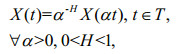 (1)
(1)then, X(t) is a single fractal, where H is the Holder index that does not change over time and does not include the local properties at a certain moment. The equal sign indicates that the finite dimensional distributions are equal.
Fractal self-affinity means that the structures of fractal objects are similar irrespective of scale. This similarity is reflected between the part and the whole system, or between any individual parts. Scale invariance means that for any part of a fractal object, whether reduced or enlarged, any new diagram maintains its characteristics and properties.
The fractal dimension is an important parameter for describing the measurement and irregularity of fractal objects. It indicates the roughness of a fractal, which is usually not an integer. If a fractal object is a time series, the fractal dimension describes how uneven the data are; if it is a space, the fractal dimension describes how the space is filled (Mao et al., 2016; Wang et al., 2017b).
Studies have shown that most natural phenomena follow the 'random walk with deviation' law (Wang et al., 2017a). The general expression of Hurst's law is as follows.
Definition 2: When a time series {x(t)}, t=1, 2, …… is considered, for any positive integer τ, there is empirically
 (2)
(2)where H is a constant that is located in the [0, 1] interval, known as the Hurst exponent, and the symbol "~" represents the direct ratio. The logarithms are taken on both sides of Eq.2 to obtain the Hurst exponent with the least squares' method. Here, R and S represent the range and the mean square deviation, respectively, which are defined as
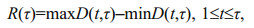 (3)
(3)and
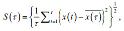 (4)
(4)where D(t, τ) is the accumulated deviation.
According to Eqs.3 and 4, R/S is a dimensionless empirical statistical characteristic quantity. Therefore, the Hurst law, as expressed in Eq.2, can relate the observation results of different timescales. Specifically, it can infer large-scale statistical rules from small-scale observation results. If the Hurst exponent values are different, the trends corresponding to the time series are different. For example, when, H=1/2, the sequence belongs to the random walk process and the sequences are unrelated. Conversely, when 1/2 < H < 1 and 0 < H < 1/2, the sequence trends are enhanced or diminished, respectively, i.e., the sequences are related and belong to the random walk with deviation process. The Hurst exponent has been used widely in research into the measurement of sequence correlation and trend intensity.
Definition 3: If there is a random process BH(t), it is continuous and it meets the criterion:
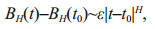 (5)
(5)where t and t0 are two different moments, H is a parameter, and 0≤w≤1. Then, the random process BH(t) is called the fractional Brownian motion and the symbol "~" represents the direct ratio.
Fractional Brownian motion is one of the Markov random processes, which can be generated by developing a random walk model (Li and Burgueño, 2010; Cai and Shi, 2016; Cai et al., 2016a, b, c; Barrs and Chen, 2018; Deng et al., 2018, 2017b, c; Kang, 2018a, b). A parameter value of H=0.5 reflects ordinary Brownian motion. The difference between Brownian motion and fractional Brownian motion is that the increment in Brownian motion is independent, whereas the increment in fractional Brownian motion is not.
Fractional Brownian motion is characterized by using a statistical law of a previous moment to relate a future changing trend (Cai et al., 2016b; Zhang et al., 2018b). Without loss of generality, when BH(0)=0, the relevant function c(t) is:
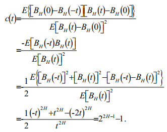 (6)
(6)According to the relationship between parameter H and correlation coefficient c(t), there are three types of time series motion: (ⅰ when H=1/2 and c(t)=0, the sequence is independent and it is a random process with an independent increment; (ⅱ) when 1/2 < H < 1 and c(t)>0, the sequence is positively correlated; and (ⅲ) when 0 < H < 1/2 and c(t) < 0, the sequence is negatively correlated. In an empirical problem, R/S analysis of a time series is conducted to determine whether it belongs to fractional Brownian motion through the Hurst index value, and to study further the correlation between the sequences.
3 GENERALIZED EXTREME VALUE PARETO DISTRIBUTION MODELIn risk assessment for flood control projects in coastal estuary cities, selecting the appropriate design flood distribution model is crucial. In this section, we established the Gumbel-Pareto distribution (GPD), i.e., a new model for design flood calculation, and we provided an explicit analytical expression of the GPD for practical applications in design flood projects.
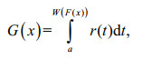
Theorem: We assume random variable T is a continuous random variable that is defined in the interval [a, b] and which uses r(t) as a probability density function. When -∞≤a < b≤∞, x is a random variable with f(x) as the density function, the distribution function is F(x), and the distribution function G(x) exists, which can be expressed as:
 (7)
(7)Proof: Alzaatreh provided a method for the generation of a continuous probability distribution family (Alzaatreh et al., 2013). When discussing the distribution of random variable X, it uses random variable T as an auxiliary variable, which shows the influence of random variable T on random variable X. First, the distribution function is defined for a new distribution function family:
 (8)
(8)where W(F(x)) is a function of the distribution function F(x), which is differentiable, monotonous, and non-decreasing with W(F(x)) [a, b]. F(x) is the distribution function of random variable x. When x→ -∞, W(F(x))→a, and when x→+∞, W(F(x))→b. The distribution function G(x) can be written as G(x)=R{W(F(x))}, which is a composite function, where R(t) is the distribution function of random variable T. Apparently, G(x) is the distribution function of a distribution function family, and its density function is:
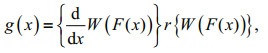 (9)
(9)where the random variable X can be discrete or continuous. Obviously, the density function r(t) of random variable T is "transformed" into a new distribution function G(x) of random variable X through the "transfer function" W(F(x)), which can be called the "T-X" distribution. G(x) shows in different forms with different W(F(x)) expressions. Without loss of generality, assuming α=0 when the range of T is [0, ∞), W(F(x)) can be defined as -log(1–(F(x)), F(x)/(1–F(x)), -log(1–Fα(x)) and Fα(x)/(1–Fα(x)), and α>0.
Specifically, when W(F(x)=-log(1–(F(x))
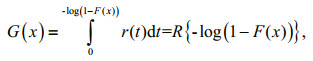 (10)
(10)where R(t) is the distribution function of random variable T. The corresponding density function of Eq.10 is:
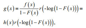
where h(x) is risk function of random variable X.
In the selection of different functions according to the actual project r(t), the corresponding g(x) can have different expressions.
Corollary 1: When r(t)=θe-θt, g(x)=θf(x)(1–F(x))θ–1
Corollary 2: When 
From Eq.7, we know that when discussing the statistical characteristics of random variable X, it takes random variable T as an auxiliary variable, which can reflect the influence of random variable T on the statistical characteristics of random variable X.
Corollary 3: If random variable T obeys the generalized extreme value distribution:
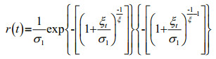 (11)
(11)then,
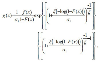 (12)
(12)where σ1 and ξ are the parameters and t≥0.
Proof: We brought Eq.11 into Eq.7 and obtained the following:
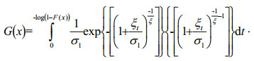
The probability density function g(x) of Eq.12 was derived from the derivation of G(x) as an explicit expression.
Corollary 4: If random variable X obeys the Pareto distribution f(x)=ασαx-α–1, α>0, x≥σ>0 where α is the shape parameter and σ is the scale parameter, which is also the threshold, Eq.12 becomes
 (13)
(13)If we make α/σ1=β, Eq.13 is simplified to:
 (14)
(14)Definition 4: If X is a random variable subject to the Pareto distribution, f(x)=ασαx-α–1, α>0, x≥σ>0, Eq.14 is called the generalized extreme value Pareto distribution, which is denoted GPD(β, σ, ξ).
Corollary 5: When random variable T is in the Gumbel distribution:
 (15)
(15)then,
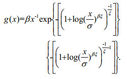
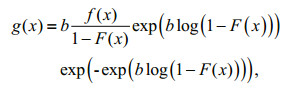 (16)
(16)where b is the parameter and t≥0. Equation 15 is brought into Eq.10 and the derivation of G(x) is undertaken.
Corollary 6: When random variable T is in the Gumbel distribution and random variable X is subject to the Pareto distribution:
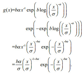 (17)
(17)Definition 5: Equation 17 indicates that random variable X obeys the GPD, which is denoted X~GPD(b, α, σ).
The characteristics of Eq.17 under different parameters are shown in Figs. 1–4.

|
| Fig.1 Probability density plots of the GPD (α=3.0, β= 0.2; 1.0; 3.0; 5.0) |

|
| Fig.2 Probability density plots of the GPD (α=3.0, 1.0; σ=5.0) |

|
| Fig.3 Probability density plots of the GPD (α=1.0, 3.0; β=1.0) |

|
| Fig.4 Probability density plots of the GPD (α=1.0, 3.0; β=3.0) |
According to the derivation process of the GPD model theory, we can see that the generalized extremevalue Pareto distribution function contains the extremevalue information of the past functional models and it combines over-threshold data, while reflecting the fractal features. The Gumbel-Pareto distribution model was applied in the engineering practice as follow.
4 EXAMPLES OF THE APPLICATION OF THE GPD MODELMost major floods in Shanghai City have been related to storm surges under the influence of typhoons and they tend to be accompanied by an upstream flood peak anstau. Therefore, we used flood volume data measured during 1970–1990 at the Wusong Hydrographic Station (Shanghai) in the Changjiang River estuary and flood observation data from the Datong Hydrographic Station 624 km upstream of Wusong. The GPD model was used to calculate the design flood for multiyear return periods, and the calculated results were compared with the value of the designed flood height calculated in the Gumbel and Pearson-Ⅲ distributions.
Figures 5 and 6 show diagnostic tests of the generalized extreme value distribution mode including charts of probability, quantile, and return level and a density histogram. The circles in the figures represent data points and solid lines represent model curves. It can be seen that the quantiles of the observation points are in good agreement with the model. The return level plot shows that when the theoretical confidence interval is 95%, the curve relationship xp–-log(-log(F(xp))) is obtained by the generalized extreme-value distribution model, which shows the distribution of the data fully within the confidence interval. The data points in the figures are distributed fully within the return level of the 95% confidence interval of the model. The density curve shows the distribution of the data intuitively, in that the observed data points (histogram) are in good agreement with the model curve.

|
| Fig.5 Flood peak anstau a. probability; b. quantile; c. return level; d. density. |

|
| Fig.6 Storm surge elevation a. probability; b. quantile; c. return level; d. density. |
The results of the above diagnostic tests show that the storm surge elevation and the corresponding upstream flood-peak anstau observation data comply with the generalized extreme value distribution and thus, can be used as an analysis sample of an extreme value distribution.
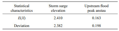
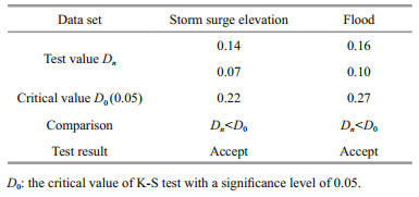
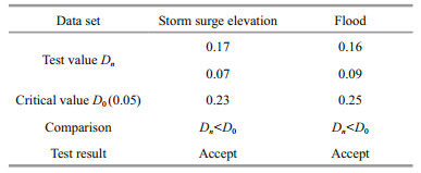
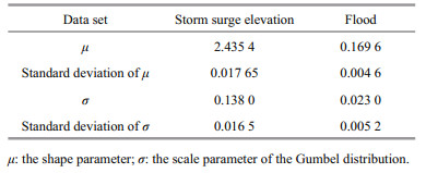
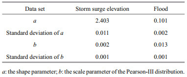
Table 1 shows the statistical values of a storm surge elevation and the flood peak corresponding upstream anstau time series. The distribution of the surge and flood sequences was normal and biased, with an extended right tail. The R/S relation was obtained using the least squares method, and the specific values of the Hurst index H, correlation function c(t), and correlation coefficient R2 are shown in Table 2. It can be seen that the storm surge elevation and flood time series are random processes with a certain trend. A fractal feature analysis of the storm surge and flood time series can be conducted using the R/S method. According to the relevance of the fractional Brownian motion trajectories, when c(t)≥0, the closer the value of H is to 1, and the stronger the long-range correlation of the time series; thus, the long-term memory of the storm surge elevation and flood time series can be obtained. In other words, if there has been a trend of increase in the past, there will be a trend of increase in the future. Conversely, if there has been a trend of decrease in the past, there will be a corresponding trend of decrease in the future. Tables 3 and 4 display the results of the K-S tests for the Gumbel and Pareto distributions of the storm surge elevation and upstream flood peak anstau. Tables 5 and 6 present the parameters and interval estimates of the 95% confidence levels when using the Gumbel distribution and Pearson-Ⅲ fitting of the storm surge elevation and flood sequences.

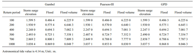
The design flood values for 100-, 200-, 400-, 500-, 700-, and 1 000-year return periods calculated using the Gumbel, Pearson-Ⅲ, and GPD distributions are shown in Table 7. It can be seen that the design flood of the multiyear return period derived from the new GPD distribution model differs a little from that derived using the common distribution. The derived design floods are generally lower than the Gumbel distribution and larger than the Pearson-Ⅲ distribution. Taking the 100- and 1 000-year return periods as examples, it can be seen that the new model is 0.06% and 1.54%, respectively, higher than the Pearson-Ⅲ distribution standard and 0.03% and 0.11%, respectively, lower than the Gumbel distribution standard. These results show that the proposed model based on fractal and extreme value theories has certain value as a reference in relation to a design flood with a 100-year return period.
1) Based on fractal and extreme value theories, this study proposed a design flood calculation model based on the GPD, and the related properties of the new model were discussed.
2) For specific parameter values, the GPD distribution was simplified into a logarithmic normal distribution and a Pareto distribution. Therefore, the GPD can include properties of both the Gumbel and Pareto distributions, highlighting a primary advantage of the new model.
3) For the calculation of a design flood, analysis methods such as fractal theory, an extreme value model, and an over-threshold model were used. However, many problems that will require further study remain. For example, the flood peak anstau and the storm surge elevation were considered as independent factors. In fact, many different combinations can constitute a 100-year return period. Therefore, a multivariable joint probability under certain controlling factor conditions will be the focus of future research.
6 DATA AVAILABILITY STATEMENTThe datasets generated and analyzed during the current study are available from the corresponding author on reasonable request.
Alzaatreh A, Lee C, Famoye F. 2013. A new method for generating families of continuous distributions. Metron, 71(1): 63-79.
DOI:10.1007/s40300-013-0007-y |
Barrs A, Chen B Y. 2018. How emerging technologies could transform infrastructure. http://www.governing.com/commentary/col-hyperlane-emerging-technologiestransform-infrastructure.html. Accessed on 2018-3-10.
|
Cai W, Huang L, Wang S. 2016a. Class D power amplifier for medical application. International Journal of Informatics Engineering, 4(2): 9-15.
DOI:10.5121/ieij |
Cai W, Huang L, Wen W J. 2016b. 2.4GHZ Class AB power amplifier for healthcare application. International Journal of Biomedical Engineering and Science, 3(2): 1-6.
|
Cai W, Huang L, Wen W J. 2017. SI-Based Class AB Power Amplifier for Wireless Medical Sensor Network. Journal of Image and Graphics, 5(1): 34-38.
DOI:10.18178/joig.5.1 |
Cai W, Shi F. 2016. High performance SOI RF switch for healthcare application. International Journal of Enhanced Research in Science, Technology & Engineering, 5(10): 23-28.
|
Chen B Y, Escalera S, Guyon I, Ponce-López V, Shah N, Simón M O. 2016. Overcoming calibration problems in pattern labeling with pairwise ratings: application to personality traits. In: Hua G, Jégou H eds. European Conference on Computer Vision (ECCV 2016)Workshops. Springer, Amsterdam, Netherlands. p.419-432, https://doi.org/10.1007/978-3-319-49409-8_33.
|
Chen B Y, Liu G L, Wang L P. 2017a. Predicting joint return period under ocean extremes based on a maximum entropy compound distribution model. International Journal of Energy and Environmental Science, 2(6): 117-126.
|
Chen B Y, Liu G L, Zhang J F. 2017b. Estimation method of designed wave height, capable of embodying influences of three typhoon factors: China Patent, CN201610972118. 2017-08-29. (in Chinese)
|
Chen B Y, Wang B Y. 2017. Location selection of logistics center in e-commerce network environments. American Journal of Neural Networks and Applications, 3(4): 40-48.
DOI:10.11648/j.ajnna.20170304.11 |
Chen B Y, Yang Z Y, Huang S Y, Du X Z, Cui Z W, Bhimani J, Xie X, Mi N F. 2017c. Cyber-physical system enabled nearby traffic flow modelling for autonomous vehicles. In: Proceedings of the 36th IEEE International Performance Computing and Communications Conference. IEEE, San Diego, California, USA. p.1-6.
|
Deng W, Yao R, Zhao H M, Yang X H, Li G Y. 2017a. A novel intelligent diagnosis method using optimal LS-SVM with improved PSO algorithm. Soft Computing, (2-4): 1-18.
|
Deng W, Zhang S J, Zhao H M, Yang X H. 2018. A novel fault diagnosis method based on integrating empirical wavelet transform and fuzzy entropy for motor bearing. IEEE Access, 6(1): 35042-35056.
|
Deng W, Zhao H M, Yang X H, Xiong J X, Sun M, Li B. 2017b. Study on an improved adaptive PSO algorithm for solving multi-objective gate assignment. Applied Soft Computing, 59: 288-302.
DOI:10.1016/j.asoc.2017.06.004 |
Deng W, Zhao H M, Zou L, Li G Y, Yang X H, Wu D Q. 2017c. A novel collaborative optimization algorithm in solving complex optimization problems. Soft Computing, 21(15): 4387-4398.
DOI:10.1007/s00500-016-2071-8 |
Escalante H J, Ponce-López V, Wan J, Riegler M A, Chen B Y, Clapés A, Escalera S, Guyon I, Baró X, Halvorsen P, Müller H, Larson M. 2016. ChaLearn joint contest on multimedia challenges beyond visual analysis: an overview. In: Proceedings of the 23rd International Conference on Pattern Recognition. IEEE, Cancun, Mexico. p.67-73.
|
Fu H L, Li Z X, Liu Z J, Wang Z L. 2018. Research on big data digging of hot topics about recycled water use on microblog based on particle swarm optimization. Sustainability, 10(7): 2488.
DOI:10.3390/su10072488 |
Fu H L, Liu X J. 2017. Research on the phenomenon of Chinese residents' spiritual contagion for the reuse of recycled water based on SC-IAT. Water, 9(11): 846.
DOI:10.3390/w9110846 |
Geng Y Y, Zhang G H, Li W Z, Gu Y, Liang R Z, Liang G Y, Wang J B, Wu Y B, Patil N, Wang J Y. 2017. A novel image tag completion method based on convolutional neural transformation. In: Proceedings of the 26th International Conference on Artificial Neural Networks.Springer, Alghero, Italy. p.539-546.
|
Hurst H E. 1951. Long-term storage capacity of reservoirs. Transactions of the American Society of Civil Engineers, 116(1): 770-799.
|
Jiang S, Lian M J, Lu C W, Gu Q H, Ruan S L, Xie X C. 2017. Prediction of the Death Toll of Environmental Pollution in China's Coal Mine Based on Metabolism-GM (1, n)Markov Model. Ekoloji, 26(101): 17-23.
|
Jiang S, Lian M J, Lu C W, Gu Q H, Ruan S L, Xie X C. 2018a.Ensemble prediction algorithm of anomaly monitoring based on big data analysis platform of open-pit mine slope. Complexity, 2018: Article ID 1048756, https://doi.org/10.1155/2018/1048756.
|
Jiang S, Lian M J, Lu C W, Ruan S L, Wang Z, Chen B Y. 2018b. SVM-DS fusion based soft fault detection and diagnosis in solar water heaters, Energy Exploration and Exploitation, https://doi.org/10.1177/0144598718816604.
|
Kang L, Du H L, Du X, Wang H.T, Ma W L, Wang M L, Zhang F B. 2018a. Study on dye wastewater treatment of tunable conductivity solid-waste-based composite cementitious material catalyst. Desalination and Water Treatment, 125: 296-301.
DOI:10.5004/dwt |
Kang L, Du H L, Zhang H, Ma W L. 2018b. Systematic research on the application of steel slag resources under the background of big data.Complexity, 2018, https://doi.org/10.1155/2018/6703908.
|
Li Z, Burgueño R. 2010. Using soft computing to analyze inspection results for bridge evaluation and management. Journal of Bridge Engineering, 15(4): 430-438.
DOI:10.1061/(ASCE)BE.1943-5592.0000072 |
Liu D F, Wang L P, Pang L. 2006. Theory of multivariate compound extreme value distribution and its application to extreme sea state prediction. Chinese Science Bulletin, 51(23): 2926-2930.
DOI:10.1007/s11434-006-2186-x |
Liu G L, Chen B Y, Wang L P, Zhang S F, Zhang K Y, Lei X. 2018. Wave height statistical characteristic analysis. Journal of Oceanology and Limnology, 36(4): 1-13.
|
Liu G L, Zheng Z J, Wang L P, Chen B Y, Dong Y J, Xu P Y, Wang J, Wang C. 2015. Power-type wave absorbing device and using method thereof: China Patent, CN105113452A. 2015-12-02. (in Chinese)
|
Mao Y, Wang J Y, Sheng B. 2016. Mobile message board: location-based message dissemination in wireless ad-hoc networks. In: Proceedings of International Conference on Computing, Networking and Communications. IEEE, Kauai, HI, USA. p.1-5.
|
Ponce-López V, Chen B Y, Oliu M, Corneanu C, Clapés A, Guyon I, Baró X, Escalante H J, Escalera S. 2016.ChaLearn LAP 2016: first round challenge on first impressions-dataset and results. In: Computer Vision -ECCV 2016 Workshops. Springer, Amsterdam. The Netherlands, https://doi.org/10.1007/978-3-319-49409-8_32.
|
Wang J Y, Wang T, Yang Z Y, Mao Y, Mi N F, Sheng B. 2017a.SEINA: a stealthy and effective internal attack in Hadoop systems. In: Proceedings of 2017 International Conference on Computing, Networking and Communications. IEEE, Santa Clara, CA, USA. p.525-530.
|
Wang L P, Chen B Y, Chen C, Chen Z S, Liu G L. 2016. Application of linear mean-square estimation in ocean engineering. China Ocean Engineering, 30(1): 149-160.
DOI:10.1007/s13344-016-0007-9 |
Wang L P, Chen B Y, Zhang J F, Chen Z S. 2013. A new model for calculating the design wave height in typhoon-affected sea areas. Natural Hazards, 67(2): 129-143.
DOI:10.1007/s11069-012-0266-6 |
Wang L P, Liu G L, Chen B Y, Wang L. 2010. New method for calculating typhoon-influenced sea area designed wave height based on maximum entropy principle: China Patent, CN201010595815. 2010-12-20. (in Chinese)
|
Wang L P, Wang L. 2011. Typhoon influence considered method for calculating combined return period of ocean extreme value: China Patent, CN102063527A. 2011-05-18. (in Chinese)
|
Wang L P, Xu X, Liu G L, Chen B Y, Chen Z S. 2017b. A new method to estimate wave height of specified return period. Chinese Journal of Oceanology and Limnology, 35(5): 1002-1009.
DOI:10.1007/s00343-017-6056-y |
Yang J Y, Zhao C, Liu G S, Xu Y. 2017. Mann-Kendall and R/S methods combined-analysis on changing trend of hydrological series-a case of Suzhou. Water Resources and Hydropower Engineering, 48(2): 27-30, 137.
(in Chinese with English abstract) |
Zhang G H, Liang G Y, Li W Z, Fang J, Wang J B, Geng Y Y, Wang J Y. 2017. Learning convolutional ranking-score function by query preference regularization. In: Proceedings of the 18th International Conference on Intelligent Data Engineering and Automated Learning.Springer, Guilin, China. p.1-8.
|
Zhang K Y, Olawoyin R, Nieto A, Kleit A N. 2018b. Risk of commodity price, production cost and time to build in resource economics. Environment, Development and Sustainability, 20(6): 2521-2544.
DOI:10.1007/s10668-017-0003-0 |
Zhang S F, Shen W, Li D S, Zhang X W, Chen B Y. 2018a. Nondestructive ultrasonic testing in rod structure with a novel numerical Laplace based wavelet finite element method. Latin American Journal of Solids and Structures, 15(7): e48.
|