 2019, Vol. 37
Institute of Oceanology, Chinese Academy of Sciences
Article Information
- XIONG Mengjie, ZHANG Jinshan, ZHANG Weisheng, YIN Chengtuan
- Heterogeneous tide-surge interaction during co-occurrence of tropical and extratropical cyclones in the radial sand ridges of the southern Yellow Sea
- Journal of Oceanology and Limnology, 37(6): 1879-1898
- http://dx.doi.org/10.1007/s00343-019-8264-0
Article History
- Received Oct. 3, 2018
- accepted in principle Jan. 3, 2019
- accepted for publication Apr. 9, 2019


2 State Key Laboratory of Hydrology, Water Resources and Hydraulic Engineering, Nanjing 210029, China
Storm surge is an abnormal rise of sea surface induced by atmospheric forcing such as extratropical cyclones or tropical cyclones. The generation of storm surge can increase the susceptibility of widespread flooding in low-lying coastal areas and damage to coastal buildings (Kerr et al., 2013; Liu et al., 2018). Jiangsu Province, China, situated at the west shore of the Yellow Sea (Fig. 1), suffers frequently from both tropical and extratropical cyclone disasters. In the past 30 years, more than 60 tropical cyclones have influenced the Jiangsu coast, in which 18 have generated large surges of more than 90 cm at Station Lüsi. Compared with typhoons, Jiangsu is more frequently attacked by extratropical cyclones and cold-air fronts, most of them are mild, but some are strong. For example, an intense extratropical cyclone during June 7–9, 2013 generated a great surface elevation of 5.18 m in the Dong-Tai coastlines, damaged the 6-km-long sea-wall armor structures and caused 10 levee collapses in the Tiaozini reclamation area, causing a direct economic loss of 5.3 million Chinese Yuan (Jiangsu Ocean & Fisheries Bureau, 2014).

|
| Fig.1 Map and bathymetry along the Jiangsu coast Red triangles indicate tide stations and yellow squares indicate the wave buoys used in model validations. T and R are abbreviations for trough and ridge, respectively. |
Tropical and extratropical cyclones have different effects on coastal dynamics. Most tropical cyclones occur from June to September, and extratropical cyclones prevail from October to May in the midlatitudes (Zhang et al., 2000). Generally, tropical cyclones always produce violent wind, higher surges but have shorter duration (less than one day) and impact small range of coastlines (~200 km). Inland flooding or inundation is potential hazard on the coastal zone. In contrast, extratropical cyclones always have lower wind speed but last for several days, affecting a larger range of more than 1 500 km of coastlines. Although accompanied by relatively lower surges, extratropical cyclones are often more destructive to the beach, dunes, and infrastructures because their storm waves can bash the shore by several high tides (Weisse et al., 2012). During the October 10–13, 2014, an extratropical cyclone event (referred to as EX1410 hereinafter) swept the Jiangsu Province. Simultaneously, the center of Typhoon Vongfong passed over the East China Sea on October 12–13 with maximum central wind speed above 38 m/s. With combined effects of the two types of cyclone processes, (40–210)-cm high surge occurred in the Nantong area and the highest water level in Station Lüsi rose to 7 cm beyond the warning level. The threatening storm surge destroyed 3 km of sea walls and bank revetments, with a direct economic loss of 20 million Chinese Yuan (Jiangsu Ocean & Fisheries Bureau, 2015). The coincidence of two cyclone systems is rare and worthy of study in the Jiangsu coast area.
Different tidal system and shelf geometry perform different interactions with storm surge. In a pioneering study of the North Sea coast and River Thames in the UK, Rossiter (1961) and Prandle and Wolf (1978) concluded that tide-surge interaction could significantly increase the magnitude of surges, especially negative and short-lived surges, and affect the timing of storm surges. More recently, tide-surge interaction has been shown to be important in many other regions worldwide, including the Meghna Estuary in Bangladesh (As-Salek and Yasuda, 2001), Northumberland Strait in the southern Gulf of St. Lawrence in Canada (Bernier and Thompson, 2007), North Sea coastline around the UK (Horsburgh and Wilson, 2007), and the northern Taiwan Strait (Zhang et al., 2010).
As one of the most striking coastal landscapes, large-scale fan-shaped radial sand ridges (abbreviated as RSRs hereinafter), covering an area of about 140 km from east to west and more than 200 km from north to south, spread over the Jiangsu coast between the abandoned Huanghe (Yellow) River estuary and the Changjiang (Yangtze) River estuary (Zhang, 2012). The RSRs consist of more than 70 sand ridges in various dimensions radiating from Jianggang towards the open sea. The RSRs area is controlled by a complex tidal system determined by the land boundaries of China and Korean Peninsula (Zhang et al., 1999). An anticlockwise rotational tidal wave system forms since a part of the tidal waves entering the southern Yellow Sea are reflected by the Shandong Peninsula. Meeting the following progressive waves from the southern Yellow Sea, the rotational waves evolve to approximately stationary tidal waves, in which the phase difference between current velocity and tidal level is about 90°. Some storm surge processes occurred during 1968–1989, including typhoons Damrey (Qi et al., 2015; Liu et al., 2017), Muifa (Yu et al., 2013), and Prapiroon (Xu, 2001), and several typical extratropical cyclone events (Zhang et al., 1999), have been simulated by many scientists. However, most of such studies focus on numerical reproduction and distribution analysis for individual surge processes. Some emphasized the sediment transport and morphological change of seabed during individual storm events. As far as we know, there are few detailed studies on kinematics characteristics and dynamic mechanisms of the tidesurge interaction behaviors in the RSRs area. Although the interaction is complex and closely associated with the local tidal motions and morphology, they deserve to be further investigated.
This research aims to investigate the surge characteristics and tide-surge interaction in the RSRs area by a coupled tide-surge-wave model. A rare simultaneous event of EX1410 and Vongfong was taken as an example. The paper is organized as follows. In Section 2, a WRF-ARW model is employed and validated to prepare high-resolution wind fields for meteorological forcing input. A coupled ADCIRC+SWAN model is established and introduced in Section 3, consisting of data source description, mesh generation, and model forcing. The model was validated by observed records of four tide gauges and two wave buoys along the Jiangsu coast. Spatial and temporal distributions of model results and different tide-surge interaction behaviors at different locations in the RSRs area are presented in Section 4. In Section 5, impacts of various factors on the degree of tide-surge interaction are discussed and dominant mechanisms are found responsible for the heterogeneousness of the interaction in the RSRs area. Conclusions are given in Section 6.
2 METEOROLOGICAL MODELING METHODOLOGY 2.1 The WRF-ARW modelThe Weather Research and Forecasting (WRF) is a mesoscale numerical weather forecasting community model capable to simulate meteorological phenomena from meters to thousands of kilometers. The WRFARW version 3.6 is implemented during the present study. It consists of fully compressible non-hydrostatic equations and the prognostic variables include the three-dimensional wind, perturbation quantities of pressure, potential temperature, surface pressure, turbulent kinetic energy and scalars. The vertical coordinate is terrain following hydrostatic pressure and the horizontal grid is Arakawa C-grid staggering.
The present model is configured in a two-way interactive nested domain. The domain configuration in WRF model for this study is shown in Fig. 2. The outer-domain has 238×286 grid points of 9-km resolution and the inner domain has 295×343 grids of 3-km resolution in the west-east and north-south directions. Thirty-five unequally spaced sigma levels are set in this model to describe vertical structures. The integral time step is 50 s. The ERA-Interim global atmospheric reanalysis data of ~80 km×~80 km grids in 60 vertical levels from the surface up to 0.1 hPa covering the entire globe every 6 h are taken as the initial and lateral boundary conditions. A third-order Runge-Kutta time integration method is used in the model.

|
| Fig.2 Nested model domain of WRF-ARW and calibration for the track of Vongfong |
The physical parameterization schemes used in this study are Kain-Fritsch (new Eta) scheme for cumulus parameterization (Kain, 2004) in the outer domain and WRF Single Moment 6-class (WSM6) scheme for microphysics (Hong and Lim, 2006), and Yonsei University (YSU) scheme for planetary boundary layer. The long-wave radiation parameterization is the Rapid Radiative Transfer Model (RRTM) scheme (Mlawer et al., 1997) and the short-wave radiation scheme is the Dudhia scheme (Dudhia, 1989). The land surface process is the Noah Land Surface Model. In addition, in order to include the negative feedback mechanism of the sea-surface temperature to the storm process, time-varying SST data are read into the model to update the sea-surface temperature field. The ocean mixed layer model based on Pollard et al. (1972) is applied to reflect atmospheric effects on the ocean in the form of wind stress and oceanic effects on the atmosphere by changed SST.
2.2 Wind field calibrationThe WRF-ARW model results are calibrated from two aspects. First, the simulated track of Typhoon Vongfong is compared with the best-moving track released by CMA in Fig. 2. Second, the modeled versus observed wind profiles at Liuting, Sheyang, Lüsi, and Pudong are shown in Fig. 3. The wind data is obtained from NCDC meteorological database. Similar typhoon tracks and wind profile curves suggest that the WRF-ARW model can output satisfying meteorological results for this event.

|
| Fig.3 Modeled versus observed wind in Liuting, Sheyang, Lüsi and Pudong |
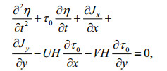
ADCIRC is a continuous-Galerkin, finite-element, shallow-water model that solves the water level and current velocity at a range of scales (Luettich et al., 1992; Luettich and Westerink, 2004). Water level is obtained from the Generalized Wave Continuity Equation (GWCE)
 (1)
(1)where
 (2)
(2)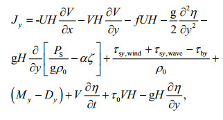 (3)
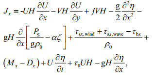
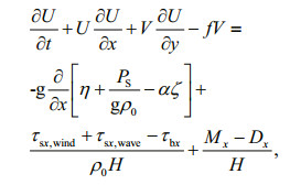
(3)and the current velocity is obtained from the verticallyintegrated momentum equations:
 (4)
(4)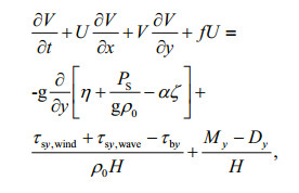 (5)
(5)where H=η+h is the total water depth (m); η is the water surface elevation (m); h is the bathymetric depth (m); U and V are depth integrated currents (m/s) in the x and y directions, respectively; f is the Coriolis parameter (s-1); g is the gravitational acceleration (m/s2); PS is the surface atmospheric pressure (Pa); ρ0 is the density of water (kg/m3); ζ is the equilibrium tidal potential (m) and α is the effective earth elasticity factor; τs, wind and τs, wave are surface stresses due to winds and waves (Pa); τb is the bed shear stress (Pa); M are lateral stress gradients (m2/s2); D are momentum dispersion terms (m2/s2); τ0 is a numerical parameter that optimizes the phase propagation properties (s-1) (Kolar et al., 1994; Atkinson et al., 2004).
SWAN simulates the wave evolution in spatial (x, y) and temporal t dimensions of the wave action density spectrum N(x, y, t, σ, θ), with σ the relative frequency and θ the wave direction (Booij et al., 1999). The governing balance equation is
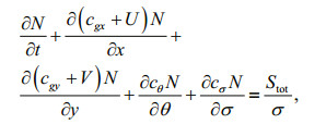 (6)
(6)where N is the wave action (J·s); cgx and cgy are the x- and y- components of the wave group velocity (m/s); σ and θ are the angular frequency and wave direction (rad); Stot is the sum of source terms (J). The source terms include wave growth by wind, action lost due to white-capping, bottom friction and surf breaking, and exchanges due to nonlinear effects between spectral components in deep and shallow water (Booij et al., 1999; Holthuijsen et al., 2003). The unstructured-mesh version of SWAN implements an analog to the fourdirection Gauss-Seidel iteration technique, maintaining SWAN's unconditional stability (Zijlema, 2010).
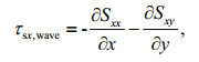
SWAN is driven by wind speeds, water levels, and currents, which are computed at the vertices by ADCIRC. The ADCIRC model is driven partially by radiation stress gradients that are computed using information from SWAN. These gradients τs, wave are computed by:
 (7)
(7)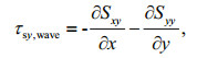 (8)
(8)where Sxx, Sxy, and Syy are the wave radiation stresses (Longuet-Higgins and Stewart, 1964; Battjes and Janssen, 1978)
 (9)
(9) (10)
(10) (11)
(11)The METIS domain-decomposition algorithm is applied to distribute the global mesh over a number of computational cores. ADCIRC and SWAN run on the same local sub-meshes and cores. The two models "leap frog" through time and exchange information from each other model. Using sweeping method, SWAN takes much larger time step than ADCIRC, whose time step is limited by Courant number due to its semi-explicit formulation, diffusion and wetting and drying algorithm. The radiation stress gradients used by ADCIRC are always extrapolated forward in time, while the wind speeds, water levels and currents used by SWAN are always averaged over each of its time steps. The integrated ADCIRC+SWAN system is highly robust because inter-model communication is intra-core, while intra-model communication is inter-core solely on adjacent sub-mesh edges (Dietrich et al., 2011).
3.2 Modeling domain and meshesThe present ADCIRC+SWAN model domain includes the Bohai Sea, the Yellow Sea and most part of the East China Sea. A total of 368 045 triangular cells with 187 332 nodes comprise the horizontal, as shown in Fig. 4. The grid resolution increases from 0.2 on the open boundary toward the study area. It becomes 1 000–1 500 m in the coast of Hangzhou Bay and about 500 m in the Changjiang (Yangtze) River estuary. The finest resolution of 100–200 m is applied in whole coastlines of the Jiangsu Province and a part of the southern waters of the Shandong Peninsula.

|
| Fig.4 Unstructured triangular mesh in ADCIRC+SWAN simulation a. the zoomed view of the computational domain; b, c. detailed meshes in the coastal areas of Lianyungang and Yangkou, respectively. |
The bathymetry data is a combination of three parts. The GEBCO bathymetry datasets are used in the open seas and the sea charts of China Navy Hydrographic Office are used in the offshore areas. Besides, valuable local underwater topographical survey data, with high spatial resolution of 50–100 m, are employed in nearshore areas of the Haizhou Bay and the southern RSRs in the Nantong region, which are prone to severe storm surge disasters.
The ADCIRC time step is 0.5 s in the storm simulation. Bottom friction is parameterized using quadratic bottom friction law and the friction coefficient Cd is varied between 0.000 2 and 0.005 4 throughout the entire domain. The coupling interval of SWAN and ADCIRC is 300 s. The SWAN frequencies range from 0.031 to 0.548 Hz and are discretized into 40 steps on a logarithmic scale. White-capping effect and quadruplet nonlinear interactions are computed. Depth-induced breaking with the breaking index γ=0.73, bottom friction based on the JONSWAP formulation and triad nonlinear interactions are computed for the shallow-water source terms.
Parallel simulation using multiple processors within the message passing environment (MPI) is implemented to shorten the run times. It takes about 10 h in DELL workstation with 32 cores of Intel Xeon CPU E5-2683 for a case of 6-day-duration storm.
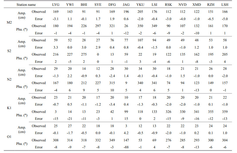
3.3 Model calibration for astronomical tideSimulations for astronomic tides are first carried out with ADCIRC to ensure the model can be employed to describe the characteristics of long-period wave propagation in the RSRs area. Eight tidal constituents (M2, S2, N2, K2, K1, O1, Q1, and P1) are forced on the open ocean boundary. The tidal constituents are derived from Naotidej.99b tidal prediction system. Table 1 and Fig. 5 shows the comparisons of modeled amplitudes and phases for five main tidal constituents (M2, S2, N2, K1, and O1) with observed ones. The semi-diurnal tides are dominant in the Yellow Sea coastline areas. The largest amplitude prediction error is -6.5 cm at RZH for the constituent M2, where the model underestimated observed values, and +4.2 cm at JAG for the constituent O1, where the model overestimated observed values. The relative amplitude errors are within ±17% in most of stations. The errors for tidal phases rarely exceed 0.5 h for semi-diurnal constituents and 1 h for diurnal constituents, except for the O1 constituent at JAG, where the modeled phase is 3 h later than the observation. The error is associated with the complicated tidal convergence pattern in the JAG, where is influenced simultaneously by a propagating tidal wave system from the East China Sea and a standing amphidromic system outside the Abandoned Huanghe River estuary. But this error produces very little effect on the modeling precision in JAG for the amplitude of O1 is only 3 cm.

|
| Fig.5 Modeled versus observed amplitude and phase for M2, K2, N2, K1, and O1 |
For storm surge simulations, the model is driven by the wind speeds, which are referred to 10 m in height, 30-min averaged, and marine exposure wind speeds, from the WRF outputs. The wind element outputs in the WRF grid every 1 h are interpolated spatially in the ADCIRC mesh by linear method. The model begins at 00:00 UTC on October 7, 2014, and ends at 00:00 UTC on October 14, 2014. The model hindcast results are validated in the duration of the simultaneous tropical and extratropical storms. The surge elevations are validated at four coastal gauges (LYG, LSI, RZH, and XMD) and the wave height and period are validated at two nearshore buoys (LYG and LSH).
According to Fig. 6, the peak surge errors (model results versus observed data) are -4 cm, -11 cm, -11 cm, and 10 cm, respectively, at LYG, LSI, RZH, and XMD, suggesting relative errors smaller than 16%. Concerning the timing of the peak storm surge, the modeling results at the four stations typically have a ±1-h shift, which is acceptable in the simulation. In Fig. 7, the modeled wave periods at LYG and LSH are in good agreement with the observed curves. The modeled Hs peak at LYG is 18% higher than the observed peak, with a main reason that the measured time series points at LYG is too coarse to capture the highest Hs. Overall, the curves of modelled surge and wave are similar to the observed ones, and the ADCIRC+SWAN model is capable to reproduce the storm surge patterns in the region of Jiangsu coast.

|
| Fig.6 Modeled versus observed water level and storm surge (water level minus astronomical tide) at LYG, LSI, RZH and XMD |

|
| Fig.7 Modeled versus observed significant wave height (Hs) and mean wave period (Tmean) at LYG and LSH |
According to WRF-ARW model results, Typhoon Vongfong passed through the Ryukyu Islands and entered the East China Sea at 2:00, October 12 UTC+8. At about 18:00, the cyclone began to change its moving direction to northeast and travelled towards the mainland of Japan. At the same period, the extratropical cyclone EX1410 controlled the weather system over the Bohai Sea and the northern Yellow Sea. Figure 8a & b shows two snapshots of modeled wind field at 19:00, October 12 and 3:00 October 13, respectively. During this event, the entire Jiangsu coast was mainly covered by the extratropical cyclone system. At the 19:00 snapshot, the Vongfong cyclone reached to a position close to the Jiangsu coast, with a geographic distance of 600 km, and its outer circulation slightly affected the sea areas of the southern RSRs area and the Changjiang River estuary. The Nantong coast was controlled by north wind of about 15 m/s and the Lianyungang and Yancheng coasts by northeast wind of 15–16 m/s. At the 03:00 snapshot, Vongfong moved far away from China and hardly affected the Jiangsu coast. Wind velocity became slightly stronger (about 16 m/s) and wind direction turned north in the RSRs area.

|
| Fig.8 Snapshots of wind fields, surge residuals and wave-induced set-up at 19:00 October 12 and 03:00 October 13, respectively a, b. wind contours and vectors, shown with a 10-min averaging period and 10 m elevation; c, d. surge residual contours, computed by ηT+S+W –ηPureT; e, f. wave-driven set-up contours, computed by ηT+S+W–ηT+S. |
Figure 8c & d show the patterns of modeled surge residuals (ηT+S+W–ηPureT) in the RSRs area at two stages. Met with regional astronomical low tide, water level fell to the lowest at 19:00, October 12 and most intertidal mud flats were exposed, including the Dongsha Ridge, Tiaozini Ridge, Gaoni Ridge and some coastal flats along Rudong and Qidong coast. Surges in most coastal areas were smaller than 0.9 m and the most serious surge was generated in the shallow waters of the Lengjiasha Ridge, reaching about 1.2 m. With the water level rising to regional high tide at 3:00, October 13, most intertidal flats were flooded. As the cold north winds blew shoreward over the southern RSRs, the surge contours tended to be parallel to the Nantong coastlines. Surges along the entire coastline to the south of Jianggang were beyond 1.3 m. Severe surges of more than 1.6 m occurred in three regions: the coastlines of Jianggang, tidal flats near the Lengjiasha Ridge and the south coastlines of Qidong. According to our field investigations, most inland regions along the Jiangsu coast were protected by hundreds of kilometers of seawalls designed to defense extreme storm surges of 50-year return period. Therefore, inland flooding is not likely to appear in cyclone processes of a medium intensity as this event.
Figure 8e & f show the effects of radiation stresses on storm surges at the times of low tide and high tide. It is found that the contribution of wave-driven set-up is not evident in the RSRs area. The largest wave setup is about 0.16 m, accounting for 16% of local surge height. Two areas are prone to generate high wave set-ups: one is shallow-water area of the Xiaomiaohong Trough and the Sanshahong Trough, and another is the coastline near the Xiyang Trough.
4.2 Heterogeneousness of tide-surge interaction in the RSRs areaSurges are modulated by the moving stationary tidal wave system (Zhang et al., 1999) in this RSRs area. To investigate the tide-surge interaction characteristics, several numerical experiments have been run for coupled tide-surge, pure tide and pure surge scenarios, respectively, to separate the storm tide into three components: astronomical tide elevations (ηPureT), surge-only elevations (ηPureS) and the nonlinear interaction terms, computed by ηI=ηT+S– (ηPureT+ηPureS), where ηT+S is coupled tide-surge model result. The simulation settings are listed in Table 2.
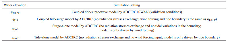
Figure 9 presents the simulated distributions of ηI in the RSRs area at four periods of low tide, mid-flood tide, high tide and mid-ebb tide in a cycle, respectively, during the EX1410 event. It shows a complex heterogeneous spatial pattern in the RSRs area. The interaction performs a quite bizarre behavior in the Xi-Yang Trough different from other locations. In most part of the southern RSRs area, ηI presents as negative on the rising tide and a slow increase to be positive on the falling tide. The value of ηI is less than 0.3 m at most of time. While, in the Xiyang Trough, high positive value of ηI emerges on the rising tide, which reaches to more than 0.6 m at the southern end of the trough at the mid-flood time, whereas ηI remains negative at other periods.

|
| Fig.9 Snapshots of tide-surge interaction residual ηI at 19:00 12th (a), 23:00 12th (b), 03:00 13th (c) and 07:00 13th (d), respectively |
To study temporal variations of the tide-surge interaction further, curves of water level, storm surges and interaction residuals at three stations Lüsi (LSI), Jianggang (JAG), and Dafeng (DFG) are shown in Fig. 10. Forced by winds of lower intensity but long duration in the EX1410 event, the storm surge set-up in the RSRs area experiences two or more astronomical tide cycles. Pure surge curves ηPureS at each station perform as slow rises and slow falls, peaking at the time of maximum local wind intensity. While, affected by nonlinear tide-surge interactions, shapes of surge residual curves (ηT+S–ηPureT) is quite different from ηPureS.

|
| Fig.10 Curves of tide level, storm surge and tide-surge interaction residual at Lüsi, Jianggang, and Dafeng stations The top figures at each station present tide level variations ηT+S in coupled model and ηPureT in astronomical tide model. The bottom figures present curves of modeled pure surge ηPureS, storm surge residual ηT+S–ηPureT and tide-surge interaction residual ηI. Green arrows above the figures denote local wind vectors. The red and blue vertical dotted lines in each figure represent the time of high tide and low tide at each station. |
The surge curves at LSI and JAG have similar properties that the interactions are closely associated with local tide level variations, performing with two features as below. First, the ηI curves show abrupt falling-down and hit bottom near every time of low tide. The minimum of ηI reaches to -0.8 m at LSI and -1 m at JAG, accounting for up to 34% of local tidal amplitudes. Second, consistent with Fig. 9, the maximum of ηI at LSI and JAG always occurs during the mid-ebb period, about 2–4 h after the time of high tide. Hence, the peak occurrence of surge residual moves closer to the time around high tide but never appears at the high tide precisely. For example, ηPureS at JAG peaks at 22:00 12th, around the time of low tide, while ηT+S peaks at 01:00 13th, about one hour before the high tide. While, at the station DFG, located at the shore of the Xiyang Trough, the performance of tide-surge interaction is quite different from the two stations above. The peak surge residual at DFG always occurs at about 4 h before the time of high tide and the value of ηI remains negative except on the early period of rising tide. Different performances of tide-surge interactions in different regions in the RSRs area suggest that they are dominated by different dynamics mechanisms, which deserve to be studied in detail in the following chapter.
5 DISCUSSION ABOUT TIDE-SURGE INTERACTION MECHANISMLarge number of studies based on observations and analysis have concluded that, many factors can affect the tide-surge interactions in coastal areas, including the state of tide, water depth variations, bottom friction, phase difference between tide and surge, and so on. In this chapter, the factors above are discussed to find out different interaction mechanisms at different locations in the coastal RSRs area.
5.1 Influence of the tidal rangeEarly simplified theoretical analyses applied to study the tide-surge interactions in the North Sea and Thames estuary (Proudman, 1955; Banks, 1974) have demonstrated that, for surge of a given magnitude, the degree of interaction is always directly proportional to the tidal range. To examine the influences of tidal range on the degree of nonlinear interactions in the RSRs area, three additional numerical experiments are conducted, under different boundary conditions of spring tide (Case Spring), neap tide (Case Neap) with the same phase but different amplitude as the real EX1410 event and middle tide of the same amplitude but reverse phase (Case Reverse) as EX1410. The tidal ranges at three stations in each experiment are listed in Table 3.

Figure 11 compares surge residual curves and interaction curves at LSI for cases of different tidal ranges (left panel) and reverse tidal phase (right panel). At LSI, the greatest fluctuation of interaction occurs in Case Spring and the slightest fluctuated curve is in Case Neap. In Case Reverse, the interaction curve makes an evident phase shift but little amplitude change. The standard deviation (STD) of ηI is employed herein to measure the fluctuation degree of tide-surge interaction. The correlation between STD of ηI and the local tidal range in the RSRs area are revealed in Fig. 12. In deep-water areas, where the still water depth is larger than 15 m, there is a good positive correlation between STD of ηI and tidal range that the correlation coefficient is 0.864 when using the least square method to fit the data. Also, most values of STD are lower than 0.1, implying that the interaction fluctuation is relatively small in deep waters. In medium-water areas, with water depth falling from 15 m to 5 m, the linear correlation is weakened progressively. Then, in shallow-water areas with water depth smaller than 5 m, scattered points are in chaos and the correlation coefficient reduces to 0.288. Hence, there is no evident correlation between the STD of interaction and tidal range.

|
| Fig.11 Curves of storm surge ηT+S–ηPureT and tide-surge interaction residual ηI at Lüsi to test the influence of tidal range (the left panel) and tidal phase shift (the right panel) |

|
| Fig.12 Standard deviation (STD) of ηI versus the local tidal range over the study area in four numerical cases The solid red line denotes the fitting curve with good agreement for SWD > 15 m and the dashed line denotes the bad fitting curve for SWD < 5 m. |
It indicates that in the RSRs area, the simple understanding of a proportional correlation between the degree of tide-surge interaction and tidal range, which is concluded from the early studies of the North Sea and Thames Estuary, is reasonable to be applied in deep-water areas, especially in troughs or open seas with water depth larger than 15 m, but inappropriate in shallow-water areas, such as over sand ridges and tidal flats.
5.2 Influence of bottom frictionSince the tidal range along most of the RSRs coastlines is typically of the order of several meters, water in tidal flats during the low tide period always becomes very shallow, making the effect of bottom friction distinct. Figure 13 presents the relationship between ηI and total depth H in the RSRs area. It shows that the curve of ηI versus H has an inflection point around H=1.26 m. A strong linear relationship (correlation coefficient is about 0.86) exists between ηI and H that ηI has a negative growth as the total depth decreases from 1.26 m to zero. While, if the total depth becomes larger than 1.26 m, the scattered points distribute around a yellow trend line with a very slight increase as the total depth decreases. It implies that the local bathymetry plays an important role on surge residuals, especially in extremely shallow-water areas. The cause of formation of the inflection point around H=1.26 m could be associated with the amplified effects of bed shear stresses.

|
| Fig.13 Tide-surge interaction residual ηI versus total water depth H over the study area in four numerical cases The red line and yellow line denote fitting curves of linear relationships at the left and right of H=1.26 m. |
In order to give a further interpretation, the maximum bed shear stress is averaged over area bins with different total depth bathymetries and shown as the histogram in Fig. 14. The bins account for 98% of the scattered modeled values with total water depth ranging ±0.1 m centered on the labeled value. For example, the bar at 0.5 m denotes the 98% maximum bed shear stress over areas with total depth ranging from 0.4 m to 0.6 m. It can be seen that the ratio of bed shear stress τb and total water depth H is subject to an inverse proportional function that τb has a gradual increase for H smaller than 1.5 m and a sharp growth for H smaller than 0.7 m. Similar relationship is shown in the study of Hu et al. (2018) on storm surge in Jamaica Bay during Hurricane Sandy. It reveals that bottom friction is a dominant factor to control the tide-surge interactions in broad tidal flats in the RSRs area, especially during the low tide period, when the local water depth falls below 1.5 m.

|
| Fig.14 Maximum averaged bed shear stress over area bins versus different total water depth The histogram covers 98% of the modeled values shown by scattered points. The red curve denotes a fitting curve of inverse proportional relationship. |
This can provide an explanation for the cause of the abrupt falling-down of interaction curves at LSI and JAG shown in Fig. 10. The stations LSI and JAG are both located at tidal flats. During the low tide period of the spring tide, the minimum total depth could reduce to only 0.4 m at LSI and 0.5 m at JAG, leading to pronounced increase of bed shear stresses and negative growth of tide-surge interaction shown in Figs. 10 & 11. Figure 15 confirms the linear relationship between the negative growth of ηI and bottom friction τ*=τb/U at the two stations and the correlation is a little bit stronger at JAG. While, the correlation at DFG is poor and opposite of which at LSI and JAG. A positive growth of ηI with the increase of τ* emerges at DFG and their correlation coefficient is only 0.45. It indicates that the dominated mechanism of tide-surge interaction in the Xiyang Trough is not same as LSI and JAG.

|
| Fig.15 Tide-surge interaction residual ηI versus τ* at three stations in different cases The solid red lines at LSI and JAG denote fitting curves of negative linear relationships with good agreement and the dashed line at DFG denotes a positive relationship with relatively worse agreement. |
The approach described in Horsburgh and Wilson (2007) can be applied to explain the tide-surge interaction mechanism in the Xiyang Trough. A simple mathematical model is given as an explanation for the preferential clustering of interaction residuals on the rising tide. If the observed real sea level is simplified to be a monochromatic long wave train, represented by
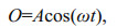 (12)
(12)and the predicted tide motion is
 (13)
(13)where A and ω are the amplitude and frequency, respectively, and φ is the phase shift between real and predicted water level, then the residual can be deduced as
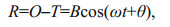 (14)
(14)where B and θ are the amplitude and phase, given by
 (15)
(15) (16)
(16)The diagrammatic sketch of O, T and R is shown in Fig. 16. As φ approaches zero,
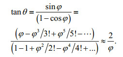 (17)
(17)

|
| Fig.16 Diagrammatic sketch of a cosine-shaped surge wave whose phase is altered but frequency and amplitude remain constant with the predicted tide wave The solid line denotes observed surge (O), the dotted line denotes predicted tide (T) and the dashed line denotes the residual obtained via subtraction (R). |
Equation 17 reveals that, if the phase shift φ between observations and predictions is positive (which means the observed surge tide travelling ahead of the predicted tide) and small enough, the tide-surge interaction residual R has a phase advance of θ≈90°, suggesting that the residual peak is at the mid-flood time on the rising tide, shown as the dashed line in Fig. 15. Conversely, if φ is negative and the observation curve lags the prediction, the residual peak will occur at the mid-ebb time on the falling tide. Anyway, modulated by tide waves with tidal range several multiples of the surge height, the phase difference between surge tide and predicted tide would not be very large in the RSRs area. According to Eq.17, the maximum interaction residual is unlikely to appear at the time of high tide mathematically, which is also reflected in Figs. 10 & 11. In addition, the study of Horsburgh and Wilson (2007) verified theoretically that the surge is prevented from peaking at high tide even at strongest meteorological forcing.
Tide and surge propagate as shallow water waves, with phase speed of (gH)1/2. It means that surge set-up can increase the total water depth H and then increase the phase speed of the real surge wave, making the surge travel faster than the predicted tide wave with a positive φ. Hence, the tide-surge interaction curve forms a positive peak in the mid-flood period several hours before the high tide and a negative trough in the mid-ebb period. This can be regarded as a simple first-order model to explain the distinct high value of interaction residuals generated in the Xiyang Trough in Fig. 9b. Analogous phenomenon of surge clustering in the rising tide period has also been observed and demonstrated along the North Sea coastline around the UK (Horsburgh and Wilson, 2007).
However, the assumption of the surge setup making the surge wave travel faster is too ideal to ignore some important factors, especially the bottom friction in shallow-water areas. Some studies pointed that the bottom friction could help to accelerate the real surge wave because it could be reduced by the surge set-up (Antony and Unnikrishnan, 2013). This positive act of bottom friction may play a role in relatively deep waters, but it is ineffective in shallow waters of the RSRs area. Different from the Xiyang Trough, the tendency that the positive ηI emerges in the mid-ebb period at LSI and JAG implies that the real surge components in large-scale tidal flats are retarded by the bottom friction effect and makes a phase lag with the tidal wave.
Our results contain some interesting conclusions for flood risk management and coastal engineering. The analysis above suggests that, peak occurrence of the surge residual will always avoid the time of high water and the significant increase of bed shear stress could help to decrease the surge height near the time of low tide in shallow waters. In addition, the tidesurge interaction tends to alleviate the flooding risk in the RSRs area around the time of high tide (and low tide), but aggravate the risk on the rising tide in the Xiyang Trough and on the falling tide in large-scale tidal flats of the southern RSRs area.
6 CONCLUSIONSpecial geometry feature and tidal system of the RSRs area in the southern Yellow Sea can result in complex storm-induced hydrodynamic patterns. To investigate the storm surge characteristics of a simultaneous event of extratropical cyclone EX1410 and Typhoon Vongfong, an integrally-coupled wave and circulation model (ADCIRC+SWAN) are implemented in this study. The meteorological forcing inputs are simulated by the WRF-ARW model. Valuable underwater topographical survey data, with high spatial resolution of 50–100 m, are employed in nearshore areas of the Haizhou Bay and the Nantong region. The simulation shows that, during 12–13, October 2014, the entire Jiangsu coast is mainly controlled by extratropical cyclone with sustained N~NE winds of 15–16 m/s. The typhoon center is more than 600 km far away from Jiangsu coast and its outer circulation has slight effects on the RSRs area. Surges of more than 1.6 m occur at three locations: the coastlines of Jianggang, tidal flats near the Lengjiasha Ridge and the south coastlines of Qidong.
Heterogeneous temporal and spatial patterns of tide-surge interaction residuals are presented in the RSRs area. The interaction residuals of LSI and JAG at the southern tidal flats appear to be tide-leveldominated, leading to abrupt sea level falling-downs of -0.8 m– -1 m near the time of low tide and the residual peaks always occur on the falling tide. While, in the Xiyang Trough, the residual pattern has a high positive value of more than 0.6 m on the rising tide but remains negative in other periods. Analysis indicates that, bottom friction is a dominant factor to control the tide-surge interactions in broad tidal flats in the RSRs area, especially when local water depth falls below 1.5 m. The sharp increase of bed shear stress in extremely shallow waters can not only reduce the surge residual height but also postpone the peak occurrence of ηI to several hours after the high tide. Different from that, the phase advances of real surge waves in relatively deep waters is the main cause for the unique clustering of surges on the rising tide in the Xiyang Trough.
7 DATA AVAILABILITY STATEMENTThe datasets generated and analyzed during the current study are not publicly available due to relative requirements of financially supporting projects but are available from the corresponding author on reasonable request.
Antony C, Unnikrishnan A S. 2013. Observed characteristics of tide-surge interaction along the east coast of india and the head of bay of bengal. Estuarine, Coastal and Shelf Science, 131: 6-11.
DOI:10.1016/j.ecss.2013.08.004 |
As-Salek J A, Yasuda T. 2001. Tide-surge interaction in the Meghna Estuary:most severe conditions. Journal of Physical Oceanography, 31(10): 3 059-3 072.
DOI:10.1175/1520-0485(2001)031<3059:TSIITM>2.0.CO;2 |
Atkinson J H, Westerink J J, Hervouet J M. 2004. Similarities between the quasi-bubble and the generalized wave continuity equation solutions to the shallow water equations. International Journal for Numerical Methods in Fluids, 45(7): 689-714.
DOI:10.1002/fld.700 |
Banks J E. 1974. A mathematical model of a river-shallow sea system used to investigate tide, surge and their interaction in the thames-southern north sea region. Philosophical Transactions of the Royal Society A:Mathematical, Physical and Engineering Sciences, 275(1255): 567-609.
DOI:10.1098/rsta.1974.0002 |
Battjes J A, Janssen J P F M. 1978. Energy loss and set-up due to breaking random waves. In: Proceedings of the 16th International Conference on Coastal Engineering.Hamburg: American Society of Civil Engineers.
|
Bernier N B, Thompson K R. 2007. Tide-surge interaction off the east coast of Canada and northeastern United States. Journal of Geophysical Research:Oceans, 112(C6): C06008.
|
Booij N, Ris R C, Holthuijsen L H. 1999. A third-generation wave model for coastal regions:1. Model description and validation. Journal of Geophysical Research:Oceans, 104(C4): 7 649-7 666.
DOI:10.1029/98JC02622 |
Dietrich J C, Zijlema M, Westerink J J, Holthuijsen L H, Dawson C, Luettich Jr R A, Jensen R E, Smith J M, Stelling G S, Stone G W. 2011. Modeling hurricane waves and storm surge using integrally-coupled, scalable computations. Coastal Engineering, 58(1): 45-65.
|
Dudhia J. 1989. Numerical study of convection observed during the winter monsoon experiment using a mesoscale two-dimensional model. Journal of the Atmospheric Sciences, 46(20): 3 077-3 107.
DOI:10.1175/1520-0469(1989)046<3077:NSOCOD>2.0.CO;2 |
Holthuijsen L H, Herman A, Booij N. 2003. Phase-decoupled refraction-diffraction for spectral wave models. Coastal Engineering, 49(4): 291-305.
DOI:10.1016/S0378-3839(03)00065-6 |
Hong S Y, Lim J O J. 2006. The WRF single-moment 6-class microphysics scheme (WSM6). Journal of the Korean Meteorological Society, 42(2): 129-151.
|
Horsburgh K J, Wilson C. 2007. Tide-surge interaction and its role in the distribution of surge residuals in the North Sea. Journal of Geophysical Research:Oceans, 112(C8): C08003.
|
Hu K, Chen Q, Wang H, Hartig E K, Orton P M. 2018. Numerical modeling of salt marsh morphological change induced by Hurricane Sandy. Coastal Engineering, 132: 63-81.
DOI:10.1016/j.coastaleng.2017.11.001 |
Jiangsu 908 Special Project Team. 2012. Comprehensive Investigation and Assessment Report of Jiangsu Offshore.Science Press, Beijing, China. (in Chinese)
|
Jiangsu Ocean & Fisheries Bureau. 2014. Ocean Disaster Bulletin Report of Jiangsu Province, 2013. (in Chinese)
|
Jiangsu Ocean & Fisheries Bureau. 2015. Ocean Disaster Bulletin Report of Jiangsu Province, 2014. (in Chinese)
|
Kain J S. 2004. The Kain-Fritsch convective parameterization:an update. Journal of Applied Meteorology, 43(1): 170-181.
DOI:10.1175/1520-0450(2004)043<0170:TKCPAU>2.0.CO;2 |
Kerr P C, Donahue A S, Westerink J J, Luettich Jr R A, Zheng L Y, Weisberg R H, Huang Y, Wang H V, Teng Y, Forrest D R, Roland A, Haase A T, Kramer A W, Taylor A A, Rhome J R, Feyen J C, Signell R P, Hanson J L, Hope M E, Estes R M, Dominguez R A, Dunbar R P, Semeraro L N, Westerink H J, Kennedy A B, Smith J M, Powell M D, Cardone V J, Cox A T. 2013. U.S. IOOS coastal and ocean modeling testbed:inter-model evaluation of tides, waves, and hurricane surge in the Gulf of Mexico. Journal of Geophysical Research:Oceans, 118(10): 5 129-5 172.
DOI:10.1002/jgrc.20376 |
Kolar R L, Gray W G, Westerink J J, Luettich R A. 1994. Shallow water modeling in spherical coordinates:equation formulation, numerical implementation, and application. Journal of Hydraulic Research, 32(1): 3-24.
DOI:10.1080/00221689409498786 |
Liu Q R, Ruan C Q, Zhong S, Li J, Yin Z H, Lian X H. 2018. Risk assessment of storm surge disaster based on numerical models and remote sensing. International Journal of Applied Earth Observation and Geoinformation, 68: 20-30.
DOI:10.1016/j.jag.2018.01.016 |
Liu W J, Li R J, Lin X, Dong X T, Li Y T. 2017. Numerical simulation of storm surge caused by Typhoon Damrey in Jiangsu sea area. Port & Waterway Engineering, (3): 22-27, 64.
(in Chinese with English abstract) |
Longuet-Higgins M S, Stewart R W. 1964. Radiation stresses in water waves; a physical discussion, with applications. Deep Sea Research and Oceanographic Abstracts, 11(4): 529-562.
DOI:10.1016/0011-7471(64)90001-4 |
Luettich R A Jr, Westerink J J, Scheffner N W. 1992. ADCIRC: An Advanced Three-Dimensional Circulation Model for Shelves, Coasts, and Estuaries, Report 1: Theory and Methodology of ADCIRC-2DDI and ADCIRC-3DL.Technical Report DTIC Document. US Army Corps of Engineers, Washington.
|
Luettich R A Jr, Westerink J. 2004. Formulation and Numerical Implementation of the 2D/3D ADCIRC Finite Element Model Version 44.
|
Mlawer E J, Taubman S J, Brown P D, Iacono M J, Clough S A. 1997. Radiative transfer for inhomogeneous atmospheres:RRTM, a validated correlated-k model for the longwave. Journal of Geophysical Research:Atmospheres, 102(D14): 16 663-16 682.
DOI:10.1029/97JD00237 |
Pollard R T, Rhines P B, Thompson R O R Y. 1972. The deepening of the wind-Mixed layer. Geophysical Fluid Dynamics, 4(1): 381-404.
DOI:10.1080/03091927208236105 |
Prandle D, Wolf J. 1978. The interaction of surge and tide in the North Sea and River Thames. Geophysical Journal of the Royal Astronomical Society, 55(1): 203-216.
DOI:10.1111/j.1365-246X.1978.tb04758.x |
Proudman J. 1955. The propagation of tide and surge in an estuary. Proceedings of the Royal Society A:Mathematical and Physical Sciences, 231(1184): 8-24.
DOI:10.1098/rspa.1955.0153 |
Qi Q H, Zhu Z X, Wang Z G, Xiong W, Chen Y C, Pang L. 2015. Numerical simulation of storm surge induced by Typhoon Dawei in Lianyungang seas. Hydro-Science and Engineering, (5): 60-66.
(in Chinese with English abstract) |
Rossiter J R. 1961. Interaction between tide and surge in the Thames. Geophysical Journal International, 6(1): 29-53.
DOI:10.1111/j.1365-246X.1961.tb02960.x |
Weisse R, von Storch H, Niemeyer H D, Knaack H. 2012. Changing North Sea storm surge climate:an increasing hazard?. Ocean & Coastal Management, 68: 58-68.
|
Xu J C. 2001. The effect of Typhoon Prapiroon on the tidal level of the Huangpu River and its research. Marine Forecasts, 18(1): 1-10.
(in Chinese with English abstract) |
Yu L L, Lu P D, Chen K F. 2013. Research on storm surge during Typhoon "Muifa" in radial sand ridges off Jiangsu coast. The Ocean Engineering, 31(3): 63-69.
(in Chinese with English abstract) |
Zhang C K, Zhang D S, Zhang J L, Wang Z. 1999. Tidal current-induced formation-storm-induced change-tidal current-induced recovery:interpretation of depositional dynamics of formation and evolution of radial sand ridges on the Yellow Sea seafloor. Science in China Series D:Earth Sciences, 42(1): 1-12.
|
Zhang K Q, Douglas B C, Leatherman S P. 2000. TwentiethCentury storm activity along the U.S. East coast. Journal of Climate, 13(10): 1 748-1 761.
DOI:10.1175/1520-0442(2000)013<1748:TCSAAT>2.0.CO;2 |
Zhang W Z, Shi F Y, Hong H S, Shang S P, Kirby J T. 2010. Tide-surge interaction intensified by the Taiwan Strait. Journal of Geophysical Research:Oceans, 115(C6): C06012.
|
Zijlema M. 2010. Computation of wind-wave spectra in coastal waters with SWAN on unstructured grids. Coastal Engineering, 57(3): 267-277.
DOI:10.1016/j.coastaleng.2009.10.011 |