 2020, Vol. 38
Institute of Oceanology, Chinese Academy of Sciences
Article Information
- CUI Chaoran, ZHANG Rong-Hua, WANG Hongna, WEI Yanzhou
- Representing surface wind stress response to mesoscale SST perturbations in western coast of South America using Tikhonov regularization method
- Journal of Oceanology and Limnology, 38(3): 679-694
- http://dx.doi.org/10.1007/s00343-019-9042-8
Article History
- Received Feb. 20, 2019
- accepted in principle May. 28, 2019
- accepted for publication Sep. 5, 2019


2 Center for Ocean Mega-Science, Chinese Academy of Sciences, Qingdao 266071, China;
3 University of Chinese Academy of Sciences, Beijing 100049, China;
4 Qingdao National Laboratory for Marine Science and Technology, Qingdao 266000, China;
5 State Key Laboratory of Satellite Ocean Environment Dynamics, Second Institute of Oceanography, Ministry of Natural Resources, Hangzhou 310012, China
Wind stress is a main driver of the ocean circulation and plays an important role in the ocean-atmosphere interaction. Many previous studies often concentrated on the large-scale ocean-atmosphere interaction (Zhang and Gao, 2016, 2017), and have found that a high wind stress magnitude leads to cold sea surface temperature (SST) through the enhanced latent heat flux (Xie and Philander, 1994), suggesting that there was a negative correlation between the large-scale wind stress and SST. As high-resolution measurements became available, mesoscale air-sea interactions can be studied. It is found that there is significant coupling between the ocean and atmosphere at a mesoscale scale of about 10–100 km, with mesoscale perturbations of wind stress (WSmeso) magnitude being positively correlated with those of sea surface temperature (SSTmeso).
The mesoscale coupling between wind stress and SST has been examined for several decades. For example, Sweet et al. (1981) found that the magnitude of cross-front wind stress was increased when wind was passing from cold to warm waters in the Gulf Stream. More observations in other regions also verified that the wind stress magnitude was enhanced (weakened) when the wind flowed over the warm (cold) waters (Businger and Shaw, 1984; Giordani et al., 1998). Furthermore, the satellite data confirmed that there was a positively linear relationship between WSmeso magnitude and SSTmeso (Chelton et al., 2001; Bourras et al., 2004). Based on the spatial derivation of the positive relationship between SSTmeso and WSmeso magnitude, Chelton et al. (2004) demonstrated that mesoscale perturbations of wind stress curl (Curl(WSmeso)) and divergence (Div(WSmeso)) were linearly proportional to the crosswind (∇crossSSTmeso) and downwind (∇downSSTmeso) components of SST gradient perturbations, respectively. These relations have been verified by observations and model simulations (O'Neill et al., 2005, 2010b, 2012; Chelton et al., 2007; Castelao, 2012; O'Neill, 2012; Frenger et al., 2013).
There are two mechanisms which can explain WSmeso response to SSTmeso (Small et al., 2008; Chelton and Xie, 2010; Gao et al., 2018). One is the downward momentum transport in the atmosphere. When wind flows from cold to warm water, warm SSTmeso can affect turbulent heat flux and lead to an intensification of turbulence within the atmospheric boundary layer, and thus there is an increased downward momentum transport. Subsequently, an increased WSmeso magnitude is induced over the warm flank of fronts and eddies. The second mechanism is the horizontal pressure adjustment. This mechanism is related to the changes of sea level pressure. According to observations, the negative sea level pressure perturbations are induced over the warm SSTmeso. Then, WSmeso in the upstream (downstream) of warm SSTmeso is accelerated (decelerated). Note that the spatial patterns of Div(WSmeso) corresponding to the SSTmeso are different in the two mechanisms. In the case of the downward momentum transport mechanism, a dipole pattern of the Div(WSmeso) is expected (Chelton et al., 2004). This is because when WSmeso increases over the warm SSTmeso, WSmeso diverge (converge) in the upstream (downstream) of warm SSTmeso. In contrast, a monopole pattern of the Div(WSmeso) is seen in the context of the horizontal pressure adjustment mechanism as WSmeso converge over the whole warm SSTmeso (Minobe et al., 2008). The differences in the spatial patterns of Div(WSmeso) between the two mechanisms have been the standard metric to measure which mechanism is dominant in the mesoscale SST-wind stress coupling.
Previous studies indicated that the mesoscale SSTwind stress coupling had significant effect on the atmosphere and ocean dynamics. On one hand, SSTmeso can affect the wind and cloud activity in the atmospheric boundary layer. Piazza et al. (2016) showed that the SSTmeso had an upscaling impact on the tropospheric wind and storm tracks in the Gulf Stream region. Renault et al. (2016) showed that the nearshore wind shape could be modulated by SSTmeso. On the other hand, WSmeso can affect the SSTmeso in return. Wei et al. (2017) showed that WSmeso had a negative feedback on SSTmeso by the means of surface heat flux in the Kuroshio Extension. In addition, the mesoscale SST-wind stress coupling also has great influence on the Ekman pumping. For example, Gaube et al. (2015) showed that the eddy-induced spatially variability of SST could affect the wind stress curl which was an important factor to drive the wind forced upwelling. Thus, Ekman upwelling could be influenced by the mesoscale SST-wind stress coupling in the regions with strong SSTmeso. This conclusion was verified by other studies. Seo et al. (2016) also showed that the Ekman pumping was modified by SSTmeso in the California Sea. The similar results were also found in the Arabian Sea (Seo, 2017). Furthermore, mesoscale eddy activities can also be affected by the mesoscale SST-wind stress coupling. Ma et al. (2016) showed that the eddy potential energy dissipation was strongly affected by the mesoscale SST-wind stress coupling and the Kuroshio Extension Jet could be weakened by about 20%–40% if the mesoscale SST-wind stress coupling was neglected in the eddy-resolving coupled climate model. Jin et al. (2009) applied an empirical air-sea coupled model that was constructed by the observed SST-wind stress relationship to a geographically idealized coastal upwelling system. They showed that if the mesoscale SST-wind stress coupling was included in the model, wind stress was weakened in the coastal sea area because of the cold coastal SST effect. The offshore Ekman upwelling was strengthened through the SST-induced wind stress curl. Besides, the eddy kinetic energy was reduced by about 25%.
The previous studies indicated that the coupling coefficients between WSmeso and SSTmeso derived from high spatial resolution models were weaker than observations (Bryan et al., 2010; Chelton and Xie, 2010). In particular, the correlation between WSmeso and SSTmeso from low spatial resolution models was opposite to observations (Bryan et al., 2010). The reason why the climate models cannot simulate the mesoscale SST-wind coupling well is that depicting WSmeso requires not only the high resolution but also accurate parameterizations of relevant physical processes in the marine atmospheric boundary layer. Therefore, it is necessary to represent mesoscale wind stress-induced feedback in the regions where mesoscale air-sea interactions are strong.
For example, Zhang and Busalacchi (2009) developed an empirical model to depict wind stress induced by tropical instability waves (TIW)-related SST perturbations in the eastern tropical Pacific Ocean. Using the observed data, they applied a combined singular value decomposition (SVD) analysis to the zonal high pass filtered TIW-related SST and wind stress fields. They found the SVDbased analysis technique could effectively extract TIW-induced covariability patterns in the atmosphere and ocean. However, the magnitude of reconstructed TIW-related wind stress fields was dependent on the number of SVD modes which were included in the statistical model-based simulation. Wei et al. (2017) studied the effects of the mesoscale wind stress-SST coupling on the Kuroshio extension. In their method, WSmeso was obtained directly from SSTmeso using observed coupling coefficient between WSmeso and SSTmeso and the direction of WSmeso was taken the same as the wind stress climatology. O'Neill et al. (2010a) showed that SSTmeso could modify surface wind direction significantly and the maximum of the changed direction could reach about 4°–8° in the strong boundary current regions. This means the wind direction is also a factor to be considered in approximating the wind stress vector perturbations.
The main goal of our study is to find a useful way to represent WSmeso in response to SSTmeso in the western coast of South America. The western coast of South America is a strong boundary upwelling system and hosts intense eddy and biological activity due to the complicated hydrography structure (Strub et al., 1998; Capet et al., 2008). Satellite observations have proved that there is strong mesoscale SST-wind stress coupling in this area (Oerder et al., 2016). On one hand, because SSTmeso can influence wind stress curl that is the dominant factor to generate the Ekman pumping (Bakun, 1990; Albert et al., 2010), the mesoscale SST-wind stress coupling has a great influence on the current dynamic system in this region. On the other hand, the mesoscale SST-wind stress coupling can affect the ocean mesoscale eddies which can influence the intense biological activity (Spall, 2007; Gruber et al., 2011; Gaube et al, 2015), so that the mesoscale SST-wind stress coupling feedback also has important ecosystem implication in this region. However, the mesoscale SST-wind stress coupling cannot be well simulated in the most current climate models and the regional ocean models when they are forced by prescribed wind and heat flux (Bryan et al., 2010). Subsequently, the feedback effects of the mesoscale coupling onto the ocean are not taken into account in these models adequately. This may be one of the reasons why there is a consistent warm SST bias in this region in the climate model simulations (Zuidema et al., 2016; Zhu and Zhang, 2018, 2019). To improve the model performances, it is necessary to develop a useful way to represent WSmeso that is related to SSTmeso.
Specifically, we exploit an empirical way to depict WSmeso based on the Tikhonov regularization. It can be useful to represent the mesoscale SST-Wind coupling and shed light on a better understanding of mesoscale SST-wind stress coupling feedback on the ocean dynamics. Details about the data and methods are given in Section 2. The observed characteristics of the mesoscale SST-Wind coupling in the western coast of South America are investigated in Section 3.1. The computational examples of reconstructed WSmeso are discussed in Section 3.2. We summarize our findings in Section 4.
2 DATA AND METHOD 2.1 DataThe wind stress data used in this study are obtained from Quik Scatterometer (Quik-SCAT, Version4). The SST fields are derived from the AMSR-E SST data (Version 7). The Quik-SCAT Scatterometer was launched in June 1999 and operated until November 2009 (Hoffman and Leidner, 2005). The AMSR-E SST data are available from June 2002 to September 2011. In this study, we use the 3-day averaged data during 2003–2008 period. All of the data are obtained from the Asia-Pacific Data-Research Center (APDRC) of the University of Hawaii, with the spatial resolution of 0.25°×0.25°.
2.2 LOESS methodThe mesoscale air/sea perturbations in the western coast of South America are extracted using a locally weighted regression (LOESS) method (Cleveland and Devlin, 1988). In the LOESS method, the weight equation is a tri-cubic function, and the weight increases as the two points get closer. The maximum intensity of the perturbation fields depends on the half-span parameter. Generally, the larger the halfspan parameter is, the larger perturbations we can get. In order to extract the mesoscale perturbation effectively in the western coast of South America, we conduct three sensitive experiments with different half-span parameters in the LOESS method. Figure 1 shows the mean probability distributions of SSTmeso during 2003–2008 from the outputs of the sensitive experiments. The results show that the maximum intensity of SSTmeso increases with the half-span parameter. However, when the half-span parameter is larger than 10°, the probability distribution of SSTmeso is almost the same as that with the half span parameter of 10°. Furthermore, it is found that the coupling coefficient obtained by the least square fitting of SSTmeso and WSmeso reaches its maximum when the half span parameters is taken as 10° (not shown). Hence, the half-span parameter is taken as 10° in the LOESS method in this study.

|
| Fig.1 The probability distributions of the mesoscale magnitude of SST perturbations as a function of the different half span parameters calculated in the western coast of South America The perturbation fields are derived by using the LOESS method and averaged from daily AMSR-E data during 2003-2008. |
The purpose of this study is to calculate the WSmeso from the Curl(WSmeso) and Div(WSmeso). To solve this problem, the Tikhonov regularization method is used. According to the Helmholtz theorem, the wind stress fields can be decomposed to:
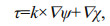 (1)
(1)in which ψ and χ are the stream function and divergent wind stress potential field, respectively; k is the vertical unit vector. Thus, the curl and divergence of the wind stress fields can be reorganized to:
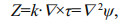 (2)
(2)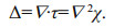 (3)
(3)The discrete version of the Eqs.2 and 3 is:
 (4)
(4)in which 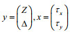
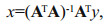 (5)
(5)in which AT is the transpose of A. Note that for the limited irregular domain, the solution may be not unique because the computation is complicated at the boundaries (Lynch, 1989). Besides, the matrix A may be ill conditioned or singular irreversible, leading to an infinite number of solutions for this problem. In these cases, the ill-posed problem can be solved effectively with the Tikhonov's regularization (Tikhonov and Arsenin, 1977). Based on the Tikhonov's regularization, the solution is:
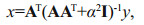 (6)
(6)in which I is the unit matrix; α is the regularization parameter. It has been found that the solution error would be rather small and acceptable when α was within the reasonable range. The α used in this study is 1.0e-6.
Li et al. (2006) computed the ocean current stream function and velocity potential from the velocity vectors by applying the regularized Tikhonov minimization procedure to the ROMS model. They found that the velocity vectors computed from the reconstructed stream function and velocity potential are almost the same as the observation. The differences between the reconstructed velocity and observation were smaller than 0.005 m/s, and the overall error was less than 1% of the observed velocity and especially small near the boundaries, which suggested that the Tikhonov method worked well at the boundary. Wei et al. (2019) also showed inverse method can produces reasonably consistent solutions compared to the one established based on the empirical relationship between WSmeso and SSTmeso in the Kuroshio Extension.
Figure 2 shows the calculation process of WSmeso with the Tikhonov regularization method, which can be summarized as follows. First, as indicated by Chelton et al. (2004), the coupling coefficient between Div(WSmeso) (Curl(WSmeso)) and ∇downSSTmeso (∇crossSSTmeso) can be obtained by the least square fitting of them based on the satellite data (in this study, the coupling coefficients are varied with month). Second, as long as we have the coupling coefficients and the SST gradient perturbations, Div(WSmeso) and Curl(WSmeso) can be obtained from SST gradient perturbations. Finally, WSmeso can be derived from Div(WSmeso) and Curl(WSmeso) by using the Tikhonov method.

|
| Fig.2 A sketch of procedure in calculating wind stress perturbation response to SST perturbations using the Tikhonov regularization method |
Although Jin et al. (2009) calculated the wind stress from the related SST using the Tikhonov method, their computational example was in the geographically idealized coastal upwelling system, which did not provide the details of reconstructed WSmeso separately. Therefore, our study focuses on the computation of the WSmeso that is highly related to SSTmeso.
3 RESULT 3.1 The observed mesoscale SST-wind stress coupling characteristicsFigure 3a shows the spatial patterns of SSTmeso (colors) in April 2007 which are derived from the LOESS filter. It indicates that SSTmeso can be well extracted by the LOESS filter. The SSTmeso fields are characterized by the alternating positive and negative bands, and the regions with high SSTmeso magnitude are in the nearshore area. The horizontal distributions of the standard deviation for high pass filtered SST are shown in Fig. 4a & b. In winter (July–October), the regions with high standard deviation for SSTmeso cover the whole area and the magnitude of standard deviation for SSTmeso in the Peru Sea is almost the same as that in the Chile Sea (Fig. 4a). In summer (December–February), the regions with high standard deviation for SSTmeso are only in the nearshore area and the magnitude of standard deviation for SSTmeso in the Chile Sea is stronger than that in the Peru Sea (Fig. 4b). In both seasons, the standard deviation for SSTmeso is small in the south-western part of the study area.

|
| Fig.3 Spatially high pass filtered wind stress and SST field in April 2007 a. Quik-SCAT wind stress magnitude (contours) and AMSR-E SST (colors); b. wind stress divergence (contours) and downwind SST gradient (colors); c. wind stress curl (contours) and crosswind SST gradient (colors). The crosswind and downwind SST gradient perturbations are in the unit of 0.1℃ per 100 km. The contour interval is 0.006 N/m2 in (a), 0.8 N/m2 per 10000 km in (b) and (c). The zero contours are omitted. |

|
| Fig.4 Horizontal distributions of the standard deviation for the high pass filtered AMSR-E SST fields in winter (a) and summer (b) that averaged during 2003–2008; correlations between the spatially high-pass filtered AMSR-E SST and Quik-SCAT wind stress magnitude in winter (c) and summer (d) The contour and shade are standard deviation for SSTmeso in (a) and (b), and correlations between SSTmeso and WSmeso in (c) and (d). The contour interval is 0.15℃ in (a) and (b), and 0.15 in (c) and (d). |
The high-pass filtered wind stress (contours) also exhibits large perturbation in the western coast of South America (Fig. 3a). The pattern of WSmeso magnitude is highly consistent with that of SSTmeso. It is evident that the wind slows down over cooler waters and speeds up over warmer waters. These relations indicate that WSmeso magnitude is positively correlated with SSTmeso. Figure 5 illustrates the timelongitude sections of spatially high pass filtered wind stress magnitude (contours) and SST (colors) along 10°S and 11.5°S. It also shows that WSmeso magnitude is positively correlated with SSTmeso. The regions with strong SSTmeso and WSmeso can stretch for a few hundred kilometers away from the shore. The relationships between SSTmeso and WSmeso are further quantified by the correlation analysis based on the satellite data during 2003–2008 (Fig. 4c & d). It shows that there is strong correlation between SSTmeso and WSmeso. The correlation patterns between SSTmeso and WSmeso are highly consistent with the patterns of standard deviation for SSTmeso (Fig. 4a & b). The regions where WSmeso and SSTmeso have high correlation are in the nearshore area in winter and the spatially averaged correlation in winter is higher than that in summer. The reason why there is higher correlation in winter may be that there is stronger wind and upwelling in Peru Sea in winter (Colas et al., 2012), which generates more mesoscale eddies.

|
| Fig.5 Time-longitude sections of the Quik-SCAT high pass filtered wind stress magnitude (contours) and AMSR-E SST (colors) along 10°S and 11.5°S The contour interval is 0.004 N/m2, with the zero contours omitted. |
In addition to WSmeso and SSTmeso, the Div(WSmeso) (Curl(WSmeso)) is also positively correlated with ∇downSSTmeso (∇cross SSTmeso) (Fig. 3b & c). The regions with large Div(WSmeso) and ∇down SSTmeso are in the nearshore area in April 2007 (Fig. 3b). The patterns of Div(WSmeso) and ∇downSSTmeso do not match very well, which may be caused by the downward momentum transport in the atmosphere and the sea level pressure adjustment. The downward momentum transport in the atmosphere and the sea level pressure adjustment are two mechanisms explaining the WSmeso response to SSTmeso, but the two processes have different effects on the distribution of Div(WSmeso) (Frenger et al., 2013). Specifically, corresponding to a monopole pattern of SSTmeso, a monopole pattern of Div(WSmeso) is induced when the pressure adjustment mechanism dominates. However, a dipole pattern of Div(WSmeso) is induced when the downward momentum transport mechanism dominates. Oerder et al. (2016) have indicated that although the mesoscale coupling was mainly forced by downward momentum transport mechanism, the near-surface pressure gradient anomalies also had a non-negligible contribution to the mesoscale coupling in the western coast of South America. Therefore, both the two mechanisms need to be considered to explain the WSmeso response to SSTmeso in the western coast of South America and affect the distribution of Div(WSmeso). As shown in Fig. 3c, the ∇crossSSTmeso is strong in the nearshore area of the Peru Sea. Because the wind stress curl is an important factor to induce the upwelling and is affected by ∇cross SSTmeso, the Ekman upwelling may be strongly influenced by the mesoscale SST-wind stress coupling in the western coast of South America.
Analyses have shown that there is strong mesoscale coupling in the western coast of South America, especially in the nearshore region. Figure 6 shows the scatterplots of WSmeso magnitude, Div(WSmeso) and Curl(WSmeso) binned by the ranges of SSTmeso, ∇down SSTmeso and ∇cross SSTmeso, respectively. The coupling coefficients are obtained from the daily data during 2003–2008. Because the mesoscale SST-wind stress coupling is weak in the southwestern part (20°S–30°S, 84°W–90°W) of the western coast of South America, the coupling coefficients in this region are not included. In Fig. 6, the top panels are the results for winter and the bottom panels are for summer; S means the coupling coefficient; black dots and vertical bars indicate the medians and interquartile ranges (IQR) in each bin. IQR is defined by difference between the upper and lower quartiles of the perturbed field. As the coupling coefficient is sensitive to some extreme values, only the central 50% of the data are specified to avoid the influences of the extreme values. It shows that there is a linear relationship between SSTmeso and WSmeso clearly (Fig. 6), indicating that Div(WSmeso) and Curl(WSmeso) can be obtained from ∇downSSTmeso and ∇crossSSTmeso, respectively. The coupling coefficient between SSTmeso and WSmeso is about 0.009 5 N/(m2∙℃) in winter and 0.008 2 N/(m2∙℃) in summer. The coupling coefficients between Div(WSmeso) and ∇down SSTmeso are larger than those between Curl(WSmeso) and ∇cross SSTmeso. In all cases, the coupling coefficients in winter are larger than those in summer. These results are similar to Oerder et al. (2016). However, the coupling coefficient between Div(WSmeso) and ∇down SSTmeso in summer is larger than that in their results, which may be caused by the differences in filter method, study area, and the SST data used in the analyses.

|
| Fig.6 Scatterplots of the spatially high pass filtered Quik-SCAT wind stress binned by ranges of AMSR-E SST perturbations for (top) winter and (bottom) summer The black dots and vertical bars indicate the medians and interquartile ranges in each bin. |
The horizontal distributions of coupling coefficients between SSTmeso and WSmeso in summer and winter are shown in Fig. 7 (The unit of coupling coefficients is N/(m2∙100℃). The distributions of coupling coefficients are highly consistent with correlations between the spatially high pass filtered SST and wind stress magnitude (Fig. 4c & d). Both in winter and summer, the regions with high coupling coefficients are in the nearshore area. There are also some special regions with negative coupling coefficients in summer in the northern part of Peru Sea. Figure 8 displays the time series of coupling coefficients between the spatially high pass filtered Quik-SCAT wind stress magnitude and AMSR-E SST, wind stress divergence and downwind SST gradient, and wind stress curl and crosswind SST gradient. It is clear that the three coefficients all exhibit the consistent seasonal variability. The maximum coupling coefficient between SSTmeso and WSmeso appeared in autumn in year 2003, 2006, and 2007 and winter in year 2004, 2005 and 2008.

|
| Fig.7 Horizontal distributions of the coupling coefficient between the spatially high-pass filtered AMSR-E SST and QuikSCAT wind stress magnitude in winter (a) and summer (b) The unit of the coupling coefficient is N/(m2∙100℃) and the contour interval is 0.1 N/(m2∙100℃). |

|
| Fig.8 The time series of the coupling coefficient during 2003-2008 for the spatially high-pass filtered Quik-SCAT wind stress magnitude and AMSR-E SST (a); wind stress divergence and downwind SST gradient (b); and wind stress curl and crosswind SST gradient (c) |
Clearly, there is strong mesoscale SST-wind stress coupling in the western coast of South America. However, the mesoscale SST-wind stress coupling processes in these regions cannot be well simulated in most climate models, and the regional ocean models when they are directly forced by prescribed wind and heat flux. Thus, the effects of the mesoscale coupling to the ocean may have not been taken into account adequately in these models. It is necessary to develop a method to represent WSmeso in response to SSTmeso effectively.
3.2 The computational examplesIn order to calculate the zonal and meridional components of WSmeso, the Tikhonov's regularization method is applied in this study with the computational procedure summarized in Section 2.
To verify the reliability of the Tikhonov's regularization method in the real cases, the WSmeso calculated from Div(WSmeso) and Curl(WSmeso) is compared with the WSmeso originally obtained from the high pass filtered wind stress. For convenience, Div(WSmeso) and Curl(WSmeso) used in the verification are directly derived from the Quik-SCAT wind data. An example is shown in Fig. 9. The left panels are the spatially high pass filtered Quik-SCAT zonal and meridional wind stress in April 2007. The right panels are the reconstructed zonal and meridional WSmeso which are derived from the observed Div(WSmeso) and Curl(WSmeso) in April 2007. It shows that the patterns of reconstructed WSmeso are highly consistent with the original WSmeso. The regions with relatively large error are mainly in the nearshore area, but the overall error is less than the 1% of the observed WSmeso, indicating that the Tikhonov's regularization method is an accurate way to compute WSmeso from Div(WSmeso) and Curl(WSmeso). We have also tried to use the SVD method to represent WSmeso, but the results (not show) are not as good as that of the LOESS and Tikhonov regularization method in the west coast of South America.

|
| Fig.9 The distributions of wind stress perturbations in April 2007 a, c. spatially high pass filtered Quik-SCAT zonal and meridional wind stress; b, d. the zonal and meridional winds stress perturbations that derived from the Quik-SCAT wind stress curl and divergence perturbations. |
So far, the reliability of this Tikhonov regularization method has been verified. Based on this method, we reconstruct WSmeso from∇down SSTmeso and∇cross SSTmeso in April 2007. The results (not shown) indicate that the magnitude of reconstructed WSmeso is weaker than the observed WSmeso. The error may be related to the coupling relationships between Div(WSmeso) (Curl(WSmeso)) and ∇down SSTmeso (∇cross SSTmeso), which are gained from the observed data. As the coupling coefficients are obtained from the linear regression method with daily data during years, the coupling coefficients may be underestimated in some regions. Besides, the Tikhonov regularization parameter may also induce small errors to the results. Both reasons mentioned above may lead to the weak magnitude of reconstructed WSmeso.
To reduce the error caused by the coupling relationships, it is necessary to make a correction to the reconstructed WSmeso. The standard deviations of the observed and reconstructed WSmeso magnitudes during 2003–2008 are calculated (Fig. 10). The regions where the standard deviations of the reconstructed and observed WSmeso have high values are both in the nearshore area of Peru Sea, and the spatially averaged maximum standard deviation in the observations is almost 2.2 times larger than that in the reconstructed WSmeso. To rescale the reconstructed WSmeso magnitude back to the corresponding observations, the magnitude of reconstructed WSmeso is multiplied by 2.2. With this correction, the magnitude of new reconstructed WSmeso derived from ∇down SSTmeso and ∇cross SSTmeso is closer to the observations. The probability distributions of the original, rescaled reconstructed WSmeso and observed WSmeso are calculated and averaged with daily data from 2003 to 2008 (Fig. 11). It shows that the probability distributions of the rescaled reconstructed WSmeso are highly similar to those of the observed WSmeso. The new reconstructed WSmeso derived from ∇down SSTmeso and ∇cross SSTmeso in April 2007 is displayed in Fig. 12. It shows that the magnitude of reconstructed WSmeso is comparable to the observed WSmeso (Fig. 9a & c), and the patterns of reconstructed WSmeso are highly consistent with those of the observed WSmeso. By comparing with the patterns of SSTmeso in April 2007 (shown in Fig. 3a), it is found that the patterns of reconstructed WSmeso are highly consistent with those of SSTmeso, indicating that WSmeso can be well represented by the Tikhonov regularization method. The regions with relative high difference between reconstructed wind stress perturbations and observation are mainly in the nearshore area.

|
| Fig.10 Horizontal distributions of the standard deviation for the Quik-SCAT wind stress magnitude perturbations during 2003–2008 (a); the reconstructed wind stress magnitude perturbations (b) The contour interval is 0.001 6 N/m2 with the zero contours omitted. |

|
| Fig.11 The probability distributions of the mesoscale perturbations of zonal (a) and meridional (b) wind stress during 2003–2008 |

|
| Fig.12 The distributions of wind stress perturbations in April 2007 a, d. reconstructed zonal and meridional wind stress perturbations which are derived from the downwind and crosswind component of the SST gradient perturbations; b, e. the difference between rescaled reconstructed wind stress perturbations and observation; c, f. the difference between original reconstructed wind stress perturbations and observation. |
Another example is shown for February 2005 (Fig. 13). The results show that the patterns of reconstructed WSmeso are almost consistent with those of the observed WSmeso. Meanwhile, the main characteristics of the observed WSmeso can also be well represented by the Tikhonov regularization method, especially in the nearshore regions. In general, the Tikhonov regularization method is an effective way to represent WSmeso in response to SSTmeso. Furthermore, the meridional and zonal WSmeso can be separately calculated, which is another important advantage of using this method.

|
| Fig.13 The distributions of wind stress perturbations in February 2005 a, c. spatially high pass filtered Quik-SCAT zonal and meridional wind stress; b, d. reconstructed zonal and meridional wind stress perturbations that derived from the downwind and crosswind component of the SST gradient perturbations. |
In this work, the relationship between SSTmeso and WSmeso in the western coast of South America is quantified based on satellite data. To extract the mesoscale perturbation field, a locally weighted regression (LOESS) method with the half-span parameter of 10° is used. The results show that the mesoscale perturbations of wind stress, wind stress divergence, and wind stress curl are positively correlated with the high pass filtered SST, downwind SST gradients, and crosswind SST gradients, respectively. The coupling coefficient between SSTmeso and WSmeso is about 0.009 5 N/(m2∙℃) in winter and 0.008 2 N/(m2∙℃) in summer. According to the horizontal distributions of the coupling coefficient between SSTmeso and WSmeso, it is found that the mesoscale coupling is strong in the nearshore area. The time series of three mesoscale coupling coefficients show the consistent seasonal variability and indicate that the stronger mesoscale SST-wind stress coupling in winter and autumn. All the results indicate that there is strong mesoscale SST-wind stress coupling in the western coast of South America. However, the mesoscale SST-wind stress coupling in these regions cannot be well simulated in many models currently used (Bryan et al., 2010). It is necessary to develop an effective method to represent WSmeso in response to SSTmeso.
The Tikhonov regularization method is used to compute WSmeso as a response to SSTmeso in this study. Based on the observed coupling coefficient between Div(WSmeso) (Curl(WSmeso)) and ∇down SSTmeso (∇cross SSTmeso), Div(WSmeso) and Curl(WSmeso) can be obtained from ∇down SSTmeso and ∇cross SSTmeso. Then, WSmeso can be calculated from Div(WSmeso) and Curl(WSmeso) with the Tikhonov regularization method. Results indicate there is a large difference between the magnitude of reconstructed WSmeso and observations when the coupling coefficients are obtained with daily data during 2003–2008. By comparing the spatially averaged standard deviations of reconstructed WSmeso magnitude and observations, it is found that a reasonable magnitude of WSmeso can be obtained when a rescaling factor of 2.2 is used. With the Tikhonov regularization method, the meridional and zonal WSmeso can also be calculated separately. Furthermore, the patterns of the reconstructed WSmeso are highly consistent with SSTmeso, indicating that the Tikhonov regularization method is a useful way to represent WSmeso in response to SSTmeso.
Although the computational applications of the Tikhonov regularization method in this study are located in the western coast of South America, this method can be applicable to any regions and useful for a variety of applications. One important application is to improve large-scale ocean model simulation, a similar way used in the TIW-induced wind feedback studies (Zhang and Busalacchi, 2008; Zhang, 2016). By using the Tikhonov regularization method to calculate WSmeso field, ocean models can be forced by the reconstructed WSmeso as well as the prescribed wind stress and heat flux. Thus, the feedback of the mesoscale air-sea coupling on the ocean can be included in the ocean model simulation, which would improve the ocean model simulation skills. Other applications include the studies on the mesoscale SST-wind coupling in any region. As the atmospheric processes are very complicated, it is difficult to well simulate the atmospheric wind response to SSTmeso in the climate models. The Tikhonov regularization method can be used to reconstruct the WSmeso in response to SSTmeso effectively. Thus, the feedback of the mesoscale SST-wind stress coupling on the ocean dynamics can be taken into account. Furthermore, these applications can shed light on a better understanding of the physical processes that are involved in the mesoscale SST-wind coupling.
For example, in the western coast of South America, there is a systematic warm SST bias in the climate model (Zuidema et al., 2016; Zhu and Zhang, 2018, 2019). According to the previous work, it might be caused by too little stratus cloud cover in the model simulations, and so an excessive amount of solar radiation reached the sea surface (Davey et al., 2002; Meehl et al., 2005). Besides, the warm SST bias could also be caused by the mesoscale interaction which is not adequately represented in the model simulations (Penven et al., 2005). All these studies do not take into account the effect of the mesoscale SST-wind stress coupling on the ocean. As the wind stress curl is an important factor inducing the upwelling and can be modified by the mesoscale SST gradients, the Ekman upwelling would be influenced by the mesoscale SSTwind stress coupling in the regions with strong SSTmeso signals. As has been demonstrated before, the simulated coupling coefficient between WSmeso and SSTmeso is weaker than observations in this region (Bryan et al., 2010). Then, the magnitude of Ekman pumping may be underestimated with less cold waters being pumped to the sea surface. Therefore, it is necessary to develop a way to represent mesoscale SST-wind stress coupling in the models to reduce the warm SST bias. With the Tikhonov regularization method, we can adequately calculate WSmeso in response to SSTmeso. This method allows us to study the feedback of the mesoscale SST-wind stress coupling on the ocean effectively and helps us to improve the model simulations, which will be examined in the future.
5 DATA AVAILABILITY STATEMENTAll of the data are obtained from the Asia–Pacific Data-Research Center (APDRC) of the University of Hawaii which is available at http://apdrc.soest.hawaii.edu/las/v6/dataset?catitem=1.
6 ACKNOWLEDGMENTThe authors wish to thank the anonymous reviewers for their numerous comments that helped to improve the original manuscript.
Albert A, Echevin V, Lévy M, Aumont O. 2010. Impact of nearshore wind stress curl on coastal circulation and primary productivity in the Peru upwelling system. J.Geophys. Res., 115(C12): C12033.
DOI:10.1029/2010JC006569 |
Bakun A. 1990. Global climate change and intensification of coastal ocean upwelling. Science, 247(4939): 198-201.
DOI:10.1126/science.247.4939.198 |
Bourras D, Reverdin G, Giordani H, Caniaux G. 2004. Response of the atmospheric boundary layer to a mesoscale oceanic eddy in the northeast Atlantic. J. Geophys. Res., 109(D18): D18114.
DOI:10.1029/2004JD004799 |
Bryan F O, Tomas R, Dennis J M, Chelton D B, Loeb N G, McClean J L. 2010. Frontal scale air-sea interaction in high-resolution coupled climate models. J. Climate, 23(23): 6 277-6 291.
DOI:10.1175/2010JCLI3665.1 |
Businger J A, Shaw W J. 1984. The response of the marine boundary layer to mesoscale variations in sea-surface temperature. Dyn. Atmos. Oceans, 8(3-4): 267-281.
DOI:10.1016/0377-0265(84)90012-5 |
Capet X, Colas F, McWilliams J C, Penven P, Marchesiello P. 2008. Eddies in eastern boundary subtropical upwelling systems. In: Hecht M W, Hasumi H eds. Ocean Modeling in an Eddying Regime, Volume 177. American Geophysical Union, Washington. 350p, https://doi.org/10.1029/177GM10.
|
Castelao R M. 2012. Sea surface temperature and wind stress curl variability near a cape. J. Phys. Oceanogr., 42(11): 2 073-2 087.
DOI:10.1175/JPO-D-11-0224.1 |
Chelton D B, Esbensen S K, Schlax M G, Thum N, Freilich M H, Wentz F J, Gentemann C L, McPhaden M J, Schopf P S. 2001. Observations of coupling between surface wind stress and sea surface temperature in the eastern tropical pacific. J. Climate, 14(7): 1 479-1 498.
DOI:10.1175/1520-0442(2001)014<1479:OOCBSW>2.0.CO;2 |
Chelton D B, Schlax M G, Freilich M H, Milliff R F. 2004. Satellite measurements reveal persistent small-scale features in ocean winds. Science, 303(5660): 978-983.
DOI:10.1126/science.1091901 |
Chelton D B, Schlax M G, Samelson R M. 2007. Summertime coupling between sea surface temperature and wind stress in the California Current System. J. Phys. Oceanogr., 37(3): 495-517.
DOI:10.1175/JPO3025.1 |
Chelton D B, Xie S P. 2010. Coupled ocean-atmosphere interaction at oceanic mesoscales. Oceanography, 23(4): 52-69.
DOI:10.5670/oceanog.2010.05 |
Cleveland W S, Devlin S J. 1988. Locally weighted regression:an approach to regression analysis by local fitting. J. Am. Stat.Assoc., 83(403): 596-610.
DOI:10.2307/2289282 |
Colas F, McWilliams J C, Capet X, Kurian J. 2012. Heat balance and eddies in the Peru-Chile current system. Climate Dyn., 39(1-2): 509-529.
DOI:10.1007/s00382-011-1170-6 |
Davey M, Huddleston M, Sperber K, Braconnot P, Bryan F, Chen D, Colman R, Cooper C, Cubasch U, Delecluse P, DeWitt D, Fairhead L, Flato G, Gordon C, Hogan T, Ji M, Kimoto M, Kitoh A, Knutson T, Latif M, Treut Le H, Li T, Manabe S, Mechoso C, Power S, Roeckner E, Terray L, Vintzileos A, Voss R, Wang B, Washington W, Yoshikawa I, Yu J, Yukimoto S, Zebiak S, Meehl G. 2002. STOIC:a study of coupled model climatology and variability in tropical ocean regions. Climate Dyn., 18(5): 403-420.
DOI:10.1007/s00382-001-0188-6 |
Frenger I, Gruber N, Knutti R, Münnich M. 2013. Imprint of Southern Ocean eddies on winds, clouds and rainfall. Nat.Geosci., 6(8): 608-612.
DOI:10.1038/ngeo1863 |
Gao J X, Zhang R H, Wang H N. 2019. Mesoscale SST perturbation-induced impacts on climatological precipitation in the Kuroshio-Oyashio extension region, as revealed by the WRF simulations. J. Oceanol. Limnol., 37(2): 385-397.
DOI:10.1007/s00343-019-8065-5 |
Gaube P, Chelton D B, Samelson R M, Schlax M G, O'Neill L W. 2015. Satellite observations of mesoscale eddyinduced Ekman pumping. J. Phys. Oceanogr., 45(1): 104-132.
DOI:10.1175/JPO-D-14-0032.1 |
Giordani H, Planton S, Benech B, Kwon B H. 1998. Atmospheric boundary layer response to sea surface temperatures during the SEMAPHORE experiment. J.Geophys. Res., 103(C11): 25 047-25 060.
DOI:10.1029/98JC00892 |
Gruber N, Lachkar Z, Frenzel H, Marchesiello P, Münnich M, McWilliams J C, Nagai T, Plattner G K. 2011. Eddyinduced reduction of biological production in eastern boundary upwelling systems. Nat. Geosci., 4(11): 787-792.
DOI:10.1038/ngeo1273 |
Hoffman R N, Leidner S M. 2005. An introduction to the nearreal-time QuikSCAT Data. Wea. Forecasting, 20(4): 476-493.
DOI:10.1175/WAF841.1 |
Jin X, Dong C M, Kurian J, McWilliams J C, Chelton D B, Li Z J. 2009. SST-wind interaction in coastal upwelling:oceanic simulation with empirical coupling. J. Phys.Oceanogr., 39(11): 2 957-2 970.
DOI:10.1175/2009JPO4205.1 |
Li Z J, Chao Y, McWilliams J C. 2006. Computation of the streamfunction and velocity potential for limited and irregular domains. Mon. Wea. Rev., 134(11): 3 384-3 394.
DOI:10.1175/MWR3249.1 |
Lynch P. 1989. Partitioning the wind in a limited domain. Mon.Wea.Rev., 117(7): 1 492-1 500.
DOI:10.1175/1520-0493(1989)117<1492:PTWIAL>2.0.CO;2 |
Ma X H, Jing Z, Chang P, Liu X, Montuoro R, Small R J, Bryan F O, Greatbatch R J, Brandt P, Wu D X, Lin X P, Wu L X. 2016. Western boundary currents regulated by interaction between ocean eddies and the atmosphere. Nature, 535(7613): 533-537.
DOI:10.1038/nature18640 |
Meehl G A, Covey C, McAvaney B, Latif M, Stouffer R J. 2005. Overview of the coupled model intercomparison project. Bull. Amer. Meteor. Soc., 86: 89-93.
DOI:10.1175/BAMS-86-1-95 |
Minobe S, Kuwano-Yoshida A, Komori N, Xie S P, Small R J. 2008. Influence of the Gulf Stream on the troposphere. Nature, 452(7184): 206-209.
DOI:10.1038/nature06690 |
O'Neill L W, Chelton D B, Esbensen S K, Wentz F J. 2005. High-resolution satellite measurements of the atmospheric boundary layer response to SST variations along the Agulhas return current. J. Climate, 18(14): 2 706-2 723.
DOI:10.1175/JCLI3415.1 |
O'Neill L W, Chelton D B, Esbensen S K. 2010a. The effects of SST-induced surface wind speed and direction gradients on midlatitude surface vorticity and divergence. J.Climate, 23(2): 255-281.
DOI:10.1175/2009JCLI2613.1 |
O'Neill L W, Chelton D B, Esbensen S K. 2012. Covariability of surface wind and stress responses to sea surface temperature fronts. J. Climate, 25(17): 5 916-5 942.
DOI:10.1175/JCLI-D-11-00230.1 |
O'Neill L W, Esbensen S K, Thum N, Samelson R M, Chelton D B. 2010b. Dynamical analysis of the boundary layer and surface wind responses to mesoscale SST perturbations. J. Climate, 23(3): 559-581.
DOI:10.1175/2009JCLI2662.1 |
O'Neill L W. 2012. Wind speed and stability effects on coupling between surface wind stress and SST observed from buoys and satellite. J. Climate, 25(5): 1 544-1 569.
DOI:10.1175/JCLI-D-11-00121.1 |
Oerder V, Colas F, Echevin V, Masson S, Hourdin C, Jullien S, Madec G, Lemarié F. 2016. Mesoscale SST-wind stress coupling in the Peru-Chile current system:which mechanisms drive its seasonal variability?. Climate Dyn., 47(7-8): 2 309-2 330.
DOI:10.1007/s00382-015-2965-7 |
Penven P, Echevin V, Pasapera J, Colas F, Tam J. 2005. Average circulation, seasonal cycle, and mesoscale dynamics of the Peru Current System:a modeling approach. J.Geophys. Res., 110(C10): C10021.
DOI:10.1029/2005JC002945 |
Piazza M, Terray L, Boé J, Maisonnave E, Sanchez-Gomez E. 2016. Influence of small-scale North Atlantic sea surface temperature patterns on the marine boundary layer and free troposphere:a study using the atmospheric ARPEGE model. Climate Dyn., 46(5-6): 1 699-1 717.
DOI:10.1007/s00382-015-2669-z |
Renault L, Molemaker M J, McWilliams J C, Shchepetkin A F, Lemarié F, Chelton D B, Illig S, Hall A. 2016. Modulation of wind work by oceanic current interaction with the atmosphere. J. Phys. Oceanogr., 46(6): 1 685-1 704.
DOI:10.1175/JPO-D-15-0232.1 |
Seo H, Miller A J, Norris J R. 2016. Eddy-wind interaction in the California Current System:dynamics and impacts. J.Phys. Oceanogr., 46(2): 439-459.
DOI:10.1175/JPO-D-15-0086.1 |
Seo H. 2017. Distinct influence of air-sea interactions mediated by mesoscale sea surface temperature and surface current in the Arabian Sea. J. Climate, 30(20): 8 061-8 080.
DOI:10.1175/JCLI-D-16-0834.1 |
Small R J, DeSzoeke S P, Xie S P, O'Neill L, Seo H, Song Q, Cornillon P, Spall M, Minobe S. 2008. Air-sea interaction over ocean fronts and eddies. Dyn. Atmos. Oceans, 45(3-4): 274-319.
DOI:10.1016/j.dynatmoce.2008.01.001 |
Spall M A. 2007. Effect of sea surface temperature-wind stress coupling on baroclinic instability in the ocean. J. Phys.Oceanogr, 37(4): 1092-1097.
DOI:10.1175/JPO3045.1 |
Strub P T, Mesias J M, Montecino V, Rutllant J, Salinas S. 1998. Coastal ocean circulation off western South America. In: Robinson A, Brink K eds. The Sea. Wiley, New York. p.29-67.
|
Sweet W, Fett R, Kerling J, La Violette P. 1981. Air-sea interaction effects in the lower troposphere across the north wall of the Gulf-stream. Mon. Wea. Rev., 109(5): 1 042-1 052.
DOI:10.1175/1520-0493(1981)109<1042:ASIEIT>2.0.CO;2 |
Tikhonov A N, Arsenin V Y. 1977. Solution of Ill-Posed Problems. Winston and Sons, Washington.
|
Wei Y Z, Wang H N, Zhang R H. 2019. Mesoscale wind stressSST coupled perturbations in the Kuroshio Extension. Prog. Oceanogr., 172: 108-123.
DOI:10.1016/j.pocean.2019.01.012 |
Wei Y Z, Zhang R H, Wang H N. 2017. Mesoscale wind stressSST coupling in the Kuroshio extension and its effect on the ocean. J. Oceanogr., 73(6): 785-798.
DOI:10.1007/s10872-017-0432-2 |
Xie S P, Philander S G H. 1994. A coupled ocean-atmosphere model of relevance to the ITCZ in the eastern Pacific. Tellus A:Dyn. Meteor. Oceanogr., 46(4): 340-350.
DOI:10.3402/tellusa.v46i4.15484 |
Zhang R H, Busalacchi A J. 2008. Rectified effects of tropical instability wave (TIW)-induced atmospheric wind feedback in the tropical Pacific. Geophys. Res. Lett., 35(5): L05608.
DOI:10.1029/2007GL033028 |
Zhang R H, Busalacchi A J. 2009. An empirical model for surface wind stress response to SST forcing induced by tropical instability waves (TIWs) in the eastern equatorial pacific. Mon. Wea. Rev., 137(6): 2 021-2 046.
DOI:10.1175/2008MWR2712.1 |
Zhang R H, Gao C. 2016. The IOCAS intermediate coupled model (IOCAS ICM) and its real-time predictions of the 2015-16 El Niño event. Sci. Bull., 66(13): 1 061-1 070.
DOI:10.1007/s11434-016-1064-4 |
Zhang R H, Gao C. 2017. Processes involved in the secondyear warming of the 2015 El Niño event as derived from an intermediate ocean model. Sci. China Earth Sci., 60(9): 1 601-1 613.
DOI:10.1007/s11430-016-0201-9 |
Zhang R H. 2016. A modulating effect of Tropical Instability Wave (TIW)-induced surface wind feedback in a hybrid coupled model of the tropical Pacific. J. Geophys. Res., 121(10): 7 326-7 353.
DOI:10.1002/2015JC011567 |
Zhu Y C, Zhang R H. 2018. An Argo-derived background diffusivity parameterization for improved ocean simulations in the tropical Pacific. Geophys. Res. Lett., 45(3): 1 509-1 517.
DOI:10.1002/2017GL076269 |
Zhu Y C, Zhang R H. 2019. A modified vertical mixing parameterization for its improved ocean and coupled simulations in the tropical Pacific. J. Phys. Oceanogr., 49(1): 21-37.
DOI:10.1175/JPO-D-18-0100.1 |
Zuidema P, Chang P, Medeiros B, Kirtman B P, Mechoso R, Schneider E K, Toniazzo T, Richter I, Small R J, Bellomo K, Brandt P, de Szoeke S, Farrar J T, Jung E, Kato S, Li M K, Patricola C, Wang Z Y, Wood R, Xu Z. 2016. Challenges and prospects for reducing coupled climate model SST biases in the eastern tropical Atlantic and Pacific oceans. Bull. Amer. Meteor. Soc., 97(12): 2 305-2 327.
DOI:10.1175/BAMS-D-15-00274.1 |