 2020, Vol. 38
Institute of Oceanology, Chinese Academy of Sciences
Article Information
- ZEINALI Saeed, TALEBBEYDOKHTI Nasser, DEHGHANI Maryam
- Spatiotemporal shoreline change in Boushehr Province coasts, Iran
- Journal of Oceanology and Limnology, 38(3): 707-721
- http://dx.doi.org/10.1007/s00343-019-8373-9
Article History
- Received Jan. 11, 2019
- accepted in principle May. 6, 2019
- accepted for publication Jul. 3, 2019


Shoreline has been identified as one of 27 important phenomena by the International Geographic Data Committee (IGDC) (Kuleli et al., 2011). Due to complicated behavior and dynamics of shorelines, they experience temporal and spatial changes, and evolve continuously over time (Stive et al., 2002; Miller and Dean, 2004; Stive et al., 2009). They experience both long term as well as short terms variations, caused by hydrodynamic processes, (e.g. river cycles, sea level rise), geomorphological phenomena (e.g. barrier island formation, spit development), and other factors (e.g. sudden and rapid seismic and storm events) (Scott, 2005). Shoreline changes are greatly concerned in many coastal areas (Genz et al., 2007). The study of shoreline evolution and its change rate is important for a broad range of coastal studies. These studies are mainly about shoreline advance and retreat (Chalabi et al., 2006; Qiao et al., 2018), construction planning (Mani et al., 1997), regional sediment budget (Kaminsky et al., 2000) and coastal morphodynamic prediction (Zeinali et al., 2016).
There have been so many methods in studying coastal and shoreline evolution. Each has been used in so many studies and their performances have been reported in the literature. Some of these methods could pointed out as numerical models based on historical data (Adamo et al., 2014), Monte-Carlo (Davidson et al., 2010; Banno and Kuriyama, 2014), mathematical models (Kaewpoo et al., 2012), models based on regime equations (Leont'yev, 2012) and those using data assimilation (Vitousek et al., 2017). Although these methods are very reliable and sophisticated, they might have some defects. The need for a huge amount of input data, which are mostly field data, increases the computational cost and effort for modeling. The fact that field data for shoreline modeling must usually be obtained at the same time of each year, makes some of the historically recorded data useless. In addition, recorded data should be taken along the shore on a particular time during a day, because of tidal variations. This will require a significant number of human power or a long period of data acquisition (Chen and Chang, 2009). Fairly, most of these models are site-specific and could be used for a particular area (Moosavi et al., 2016). Due to the complexity of coastal areas and the significance of affecting parameters, these models may exclude some parameters for the sake of simplification. Therefore, using a simpler method with fewer simplifications and trustable results can be advantageous.
Ground-based surveys of rapidly changing landscapes are intrinsically complicated and expensive (Mills et al., 2005). Subsequently, most of the world's coastline morphology has not been quantified sufficiently. However, improvements in coastal studies suggest that remote sensing and geographical information system (GIS) are very useful tools and make the studies easier (Yamano et al., 2006). Remote sensing enables us to record the current location of shoreline rapidly and easily as well (Addo et al., 2008). The application of satellite images simply provides images of the study area for the desired period and acquisition date (Chen and Rau, 1998; Mishra et al., 2019). In addition, these images have recorded the effect of all dominant parameters on the coastal area and shoreline. Therefore, no unnecessary simplifying assumption is required. Furthermore, the fact that the satellite images are available for any study makes it globally applicable. Finally, it can be pointed out that these valuable data can be used for change prediction, which is key information for long-term management planning.
The rate calculation is carried out by regression methods, e.g. end point rate (EPR). These methods are applied to enquire change rate statistically, over the study period based on the formulation of each method. The distance of shorelines from a userdefined baseline in different years of acquired images and their temporal intervals are the input information of these methods. Some of them include the reliability of each extracted shoreline, while others deal with all shorelines equally, and similarly. The performance of each method is the key factor to be chosen for further steps of this study. These approaches are discussed and examined widely in the literature. An automatic analytical techniques using a geographical information system (GIS) and a digital shoreline analysis system (DSAS) were applied to analyze shoreline change rates along the 20 km Kenitra coast, Morocco (Moussiad et al., 2015). Jijelian sandy coast in East Algeria was studied and the statistics of shoreline changes were illuminated thoroughly using QuickBird satellite images covering the period 1960–2014 (Kermani et al., 2016). In another study, a selfdeveloped shoreline analysis program was used to analyze shoreline changes extracted from aerial photos for southwestern France (Castelle et al., 2018) with almost 270 km of high-energy sandy coast. A similar procedure was used to analyze change rates in the Goku Delta, Turkey, where five Landsat images between 1984 and 2011 were used for shoreline extraction. Then shoreline change envelope (SCE), EP rate, and linear regression (LR) rate were the methods to calculate change rates (Ciritci and Türk, 2019).
The selected study area is of great importance in several aspects due to the diverse activities along its sandy shores. Accordingly, the core objectives of this study were to analyze shoreline changes in the study area, calculate change rates, and estimate the future position of the shoreline. The statistical results of this study could give a better understanding of the patterns of sediment movement in the area, and hopefully could be used to estimate the direction of longshore erosion and sedimentation in future studies.
2 STUDY AREABoushehr Province is located in the south Iran, on the shores of the Persian Gulf. Shorelines of this province are chosen for monitoring (Fig. 1). This region is of value because it holds subareas with industrial, economic, municipal and tourism activities. Each of these activities and communities in a coastal area is crucial enough to justify the importance of this study. Asaluyeh is the heart of oil and gas production in Iran is also located in this area. Also, other municipal communities of this region such as Shirino and Nakhl Taghi ports, are highly dependent on fishing. Furthermore, Nayband Bay is a visiting target for tourists because of clean water and diverse shoreline. Altogether, to find the nature of shoreline changes in this area can be a fundamental element for shoreline management.

|
| Fig.1 Location of the study area in Iran and along Persian Gulf beaches |
The significance of the Asaluyeh oil and gas industry has affected the area in several ways. First, the shoreline in this industrial zone has been disturbed enormously in time. Second, this industry has attracted population to neighboring urban areas. Accordingly, constructions along shores have recently increased a great deal (Ebadati et al., 2018).
The study area is from Shirino port to Haleh beach. The average annual rainfall in this area is 157.32 mm. In addition, the tidal range is 2.11 m on average, with variation from 0.7 to 3.32 m during neap and spring tides, respectively (Kalantari et al., 2012). Most of the sediment transport in this area is caused by wave diffraction and tidal currents. This area is exposed to waves traveling mostly in the northwest to southeast direction, creating longshore sediment transport. An approximate amount of 21 000 m3 sediments per year moves along the shore in this area (Sami et al., 2010).
3 MATERIAL AND METHODSatellite images are the main materials for this study, and here Landsat images with 30-m pixel size, have been used from different sensors for covering the period of the study. Satellite data over the study area for the period from 1987 to 2017 have been acquired. These data are from Landsat satellite sensors, i.e. Thematic Mapper (TM), Enhanced Thematic Mapper (ETM)+ and Operational Land Imager (OLI). The acquired data are listed in Table 1.

The next step is to extract the shoreline from each image. For this purpose, three steps must be taken. First, a water body in each image should be highlighted by the normalized difference water index (NDWI). Then the image should be divided into two categories by thresholding. Finally, shoreline must be obtained by the morphology filter as the edge of two categories. Each of these actions is explained in detail, in Section 3.1.
Then, the changes in the location of the extracted shoreline in the direction of perpendicular to shoreline must be identified. For this part, transects are introduced in constant intervals along the shoreline whose intersections with the shoreline in different dates give shoreline movement in time. Eventually, temporal changes along each transect are calculated by these locations. Net shoreline movement (NSM) is a sample of shoreline change, which indicates the change between the first and last acquired date.
Furthermore, these changes are used to calculate the rate of change along each transect, for instance, temporal changes divided by the acquired period. There exists a bulk of methods to calculate change rates, and four of them are used in this study. Results of all four methods are verified by an available shoreline and their performance is compared.
Finally, the method with the best performance is applied to calculate the shoreline position for 2050 and 2100. These steps are illustrated in Fig. 2.

|
| Fig.2 Flowchart of methodology |
There are several methods to extract shoreline in a satellite image such as visual interpretation (Winarso and Budhiman, 2001), classification (Yamani et al., 2011; Zeinali et al., 2017), band ratio and thresholding (Guariglia et al., 2006). The accuracy of visual interpretation is very dependent on the accuracy of the interpreter. This method is a subjective one with a high degree of approximation, which leads to low accuracy. On the other hand, the classification method is based on the training data selected for each class. The classification accuracy is therefore highly related to the accuracy of the training data.
For the extraction of open water features, an index, namely, the NDWI that uses two spectral channels can be applied. Consequently, the shoreline will be delineated as well. This criterion increases the contrast between water and land in an image. The NDWI is applied to every single pixel in the image (McFeeters, 1996). The resulted images are then applied by a thresholding equation. In thresholding of an image, I(x, y) contains both bright and dark objects. These objects may be differentiated by a straightforward equation called thresholding along with a value called T, that is the threshold magnitude decided statistically or empirically by the analyst. All the pixels which belong to the bright object are coded as 1, while the dark part is labeled by 0 (Singh, 1989). In order to indicate irregular objects in an image, morphological operations can be used. Morphological processing is a template-based operation that the template chosen by the operator establishes how the object in an image is modified. This template operation is defined in terms of a structuring element (SE), which is effectively a template. In this template, the elements are either present or not present, and are often represented respectively by template entries of 1 and 0. One of these operations is erosion. As its name implies this operation has the effect of eroding, and thus reducing the size of an object. Members of the structuring element are named as S while O is the set of pixels from which the object is composed. A sample SE is addressed as Si, j, in which subscripts (i, j) are the location of image pixel that the center of structuring element is placed on. The structuring element is said to be a subset of the object, if it is completely located inside the object, and it is written as Si, j⊆O. The eroded object is the set of pixels that fits into the subset condition. If the set of pixels of the eroded object is named E then that object is expressed as (Richards, 2013):
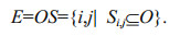 (1)
(1)The equation says that from all points of the original object, only the set of points that satisfy the subset condition (SE completely enclosed within original object) will form the eroded object. Erosion is represented by symbol. Deducing the eroded object from its original will effectively give the boundaries, since the boundaries are shrunk by erosion. This is written in the form of:
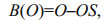 (2)
(2)where B(O) is the difference between the object and its eroded version as set of pixels (Richards, 2013).
3.2 Accuracy assessmentThe processing of remotely sensed imagery and procedures of extracting shorelines introduces errors during shoreline change analysis. Therefore, to obtain reliable shoreline change statistics, three sources of uncertainties are considered in this study, i.e., digitizing error, pixel error, and rectification error. Pixel error is calculated by the spatial resolution of the images. Georeferencing error is calculated from the standard deviation of the shoreline position from rectification, and the standard deviation of the shoreline position from repeated digitization of the same part of coast by several operators could give the interpretation error. The overall shoreline error is derived from the above errors, which is the root mean squared errors (RMSE) for each acquisition date (Table 1).
3.3 Calculation of shoreline changing rateAll of the shorelines are overlaid simultaneously and a baseline is defined in the area, manually. This baseline is considered as a reference line for further steps.
Transects perpendicular to baseline at desired spacing (100 m) is then created. These transects intersect with each shoreline, casting measurement points. The rate of changes is then computed from the distance between the baseline and the intersection points. The rate-of-change statistics include NSM, EPR, LRR, least median of squares (LMS), and weighted linear regression (WLR) rate. Digital shoreline analysis system (DSAS) (Thieler et al., 2009) by the United States Geological Survey (USGS), an extension for ArcMAP, has been employed for this purpose.
The NSM reports a distance between a single shoreline corresponding to two particular dates. These two dates are the oldest and the most recent ones and the distance values are calculated along each transect. The EPR is calculated by dividing the values of NSM by the time elapsed between two shorelines (Thieler et al., 2009).
 (3)
(3)Easy computation and requiring only two shorelines in different times are the main advantages of this method while the disadvantage is missing the major phenomenon or alteration between accretion and erosion of the shoreline in the elapsed time (Thieler et al., 2009).
A linear regression rate (LRR)-of-change statistic can be determined by fitting a least-squares regression line to all shoreline points for a particular transect, in the form of (Genz et al., 2007):
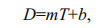 (4)
(4)where D is the distance from baseline and T is shoreline date. The LRR is the slope of the line m, and b is the gain of the fitted regression line. Then, if more reliable data are given with weight in determining a best-fit line, the method is called the weighted linear regression. The weight (w) is defined as a function of the variance in the uncertainty of the measurement (e) (Genz et al., 2007):
 (5)
(5)where e is shoreline uncertainty value. In ordinary and weighted linear regression, the best-fit line is placed through the points in such a way as to minimize the sum of squared residuals. In the linear regression method, the sample data are used to calculate a mean offset, and the equation for the line is determined by minimizing this value so that the input points are positions as close to the regression line as possible. In the LMS method the median value of the squared residuals is used instead of the mean to determine the best-fit equation for the line. This method is a more robust regression estimator that minimizes the influence of an anomalous outlier on the overall regression equation (Thieler et al., 2009).
3.4 Shoreline predictionImages acquired from 1987 to 2011 are used for computing the statistics, as in training, while the image acquired in 2017 image is considered for validating. Performance of all methods are examined by using them to estimate 2017 shoreline and comparing their result with actual location of 2017 shoreline, across each transect. The performance criteria is mean absolute percentage error (MAPE) between the estimated and actual positions of 2017 shoreline intersected at all transects. The MAPE is a measure of prediction accuracy of a forecasting method in statistics. It expresses accuracy as a percentage, and is defined as:
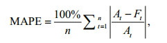
where At is the actual value and Ft is the forecast value. The difference between At and Ft is divided by the At again. The absolute value in this calculation is summed for every forecasted points and divided by the number of fitted point n. Multiplying by 100% makes it a percentage error (De Myttenaere et al., 2016).
Then it is assumed that the shoreline changes in time by the rate of the best-featured method after 2017. By that, a rough estimation of the shoreline location in 2050 and 2100 could be achieved.
4 RESULT AND DISCUSSIONThe whole process of extracting shorelines including applying the NDWI, thresholding and morphological filtering is elaborated in Fig. 3.

|
| Fig.3 Shoreline extraction for the image acquired in 2017 a. original image; b. NDWI applied on the original image; c. thresholding applied on NDWI; d. after morphological filtering. |
For more detailed monitoring of the shoreline, the study area was divided into 5 different subsets (Fig. 4a). Shorelines extracted in all acquisition dates as well as the baseline defined for all subsets are plotted on the 2017 original image (Fig. 4b). Transects were defined for the whole area for all acquisition dates. Moreover, 642 transects at 100 m intervals were automatically created along the shorelines. Latitude and longitude of top left transect are 27°38′59″N and 52°23′40″E, and those for the bottom right transect are 27°20′03″N and 52°38′44″E. The baseline was then defined on the landside of the shoreline, which is demonstrated in Fig. 4b with a black bold line. The position of shorelines on all acquisition dates along the created transects, which is measured according to the baseline, is presented in Fig. 5. Among all subsets, Nakhl Taghi shows significant sedimentation from 1999 to 2005, which is due to the massive constructions on the shoreline and building several docks in the area that moved the shoreline seaward, dramatically. Another phase of constructions seems to have moved the shoreline in the same direction between transects 145 to 165 in the 2005–2017 period.

|
| Fig.4 Subsets of the study area (a) and the shorelines extracted at acquisition dates and the defined baseline (black line) (b) |

|
| Fig.5 Position of shoreline on all acquisition dates along the created transects |
Shoreline changes along transects were calculated over the period of interest. The values of NSM are depicted in Fig. 6. It can be observed that the main accretion happens on Nakhl Taghi due to massive constructions. The magnitude of changes are categorized into different groups whose frequency are calculated in Fig. 7. In this figure, the values of the whole area are depicted in Fig. 7a, and in Fig. 7b Nakhl Taghi is excluded for better analysis. From Fig. 7a, we understand that accretion is dominant in this area (51.11%). Most of the accretion is less than 150 m and almost 13% of transects reports sedimentation more than 350 m. The maximum erosion is 360 m whereas maximum accretion is 680 m, which indicates that accretion has happened more significantly. Because of local constructions in Nakhl Taghi, if we exclude this part of shoreline from the statistics, the maximum value of accretion changes to 310 m and erosion values remain constant. In this situation, erosion is dominant (60%) (Fig. 7). Moreover, the fluctuations in shoreline position in the period between 1987 and 2011, is presented in Fig. 8. It suggests that most of the overall erosion has taken place between 1987 and 1993 and after that between 1999 and 2005. Maximum accretion, on the flip side, has happened from 1999 to 2005 and from 2005 to 2011. The construction that is talked about on the Nakhl Taghi subset has been made during the 1999– 2005 period, which is between transects 170 and 245. Also, this constructions goes on to take place on Nakhl Taghi subset during the 2005–2011 period between transects 145 to 165. Not taking into consideration these considerable changes, during two time periods 1993 to 1999 and 2005 to 2011, accretion is dominant in most of the transects, and erosion is recorded mostly in the last transects.

|
| Fig.6 Net Shoreline Movement in the study area (1987–2011) Green color shows accretion while red color shows erosion. |

|
| Fig.7 Frequency of shoreline changes a. over all 5 subsets; b. Nakhl Taghi excluded. |

|
| Fig.8 Net shoreline movements between acquired dates Green color shows accretion while red color shows erosion. |
Rate-of-change statistical approaches have widely been used to obtain reliable results in time-series studies of satellite images, despite the inconsistencies and variations in their accuracy (Douglas and Crowell, 2000; Maiti and Bhattacharaya, 2009; Santra et al., 2011). The rate-of-change along all transects extracted from different methods including EPR, LRR, WLR, and LMS were calculated (Fig. 9). As observed, the first three methods have a similar behavior in almost all of the transects. In certain parts of the shoreline, however, the LMS method resulted in different rates.

|
| Fig.9 Rate of change along all transects from all methods |
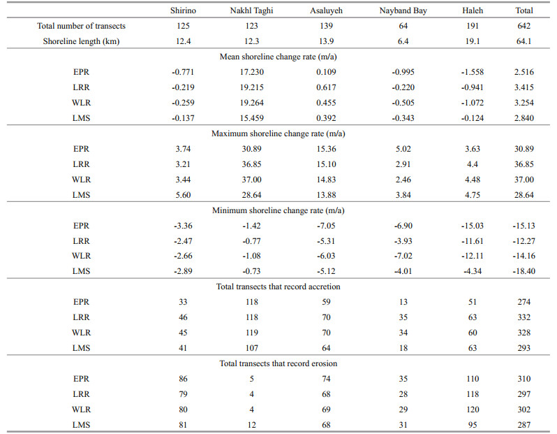
For a more detailed study of shoreline changes in this area, statistics of change rates using three methods, i.e. LRR, WLR, and LMS, are compared in all five subsets and illustrated in Figs. 10 to 14, and Table 2.

|
| Fig.10 Change rates between 1987 and 2011 calculated by LRR, WLR, and LMS for Shirino subset |

|
| Fig.11 Change rates between 1987 and 2011 calculated by LRR, WLR, and LMS for Nakhl Taghi subset |

|
| Fig.12 Change rates between 1987 and 2011 calculated by LRR, WLR, and LMS for Asaluyeh subset |

|
| Fig.13 Change rates between 1987 and 2011 calculated by LRR, WLR, and LMS for Nayband Bay subset |

|
| Fig.14 Change rates between 1987 and 2011 calculated by LRR, WLR, and LMS for Haleh subset |
All four methods were used to calculate change rates. These rates were then used to obtain the shoreline corresponding to 2017. The calculated shoreline location in 2017 and the actual one are compared for all subsets in Fig. 15.

|
| Fig.15 Estimated compared to extracted 2017 shoreline |
With respect to Figs. 10 to 14 and Table 2, it can be found out that on the Shirino sector, accretion has happened in greater rates but most of the transects experience erosion. Therefore, the mean change rate is negative. Most of the transects in the Nakhl Taghi sector are under accretion, and the main reason, as mentioned previously, is due to the construction of the oil and gas industry in this area. The mean change rate in this area is far greater than other sectors, and the maximum change rate is almost twice the rate in Asaluyeh and it is 10 times those of other sectors. These values are the results of human activities and could not be considered because of natural processes. The Asaluyeh sector starts with transects experiencing erosion and continues with accretion, which could be said that the eroded sediments in starting transects are deposited in finishing transects. It could also be verified by the previously mentioned fact that the dominant wave direction in the region is northwest to southeast. Mean change rates are almost in balance with a slight favor in accretion. However, accretion rates are greater than erosion ones. For the Nayband Bay, mean change rates are towards erosion, and maximum and minimum rates are equal. In this subset, WLR reports a balanced condition between 399 and 410 transects, unlike LRR and LMS. Finally, the Haleh sector is dominated by erosion, which has taken place in the final transects. In this sector, between transect 537 and 602; change rates are very low, which could be due to the rocky shores in this part.
For accuracy assessment of these methods, MAPE has been calculated between the available and calculated shoreline of 2017 (Table 3) and are compared in Fig. 15. As presented, the least accuracy has been achieved on Nakhl Taghi, which has experienced massive constructions over time, and it has been an anomaly to the natural evolution of shoreline. Therefore, using statistical methods may reflect results with low accuracy. However, there have been reliable results on the other subsets. Overall results showed that LMS has a fairly better result for predicting shoreline of the year 2017. Thereby, this method is used to predict long-term shoreline locations for years 2050 and 2100 (Fig. 16). A prediction has been carried out by assuming that the change rates calculated by LMS, will continuously change the location of shoreline until targeted years. Therefore, the change rates are multiplied by 33 and 83 years, and then added to the location of shoreline in 2017, in order to gain location for the years 2050 and 2100, respectively. As observed previously, changes in Nakhl Taghi are remarkable. Since these changes are made by coastal structures, it does not seem to continue to change by the same rate, so such results can be ignored in predictions. The least amount of evolutions is happening in Haleh. That is because this part of shoreline mostly includes rocks and is, therefore, resistant against sedimentation and erosion.


|
| Fig.16 Estimated future shoreline position for 2050 and 2100 with respect to defined baseline |
In Shirino, the most fluctuations are predicted near transects 21 and 66. These parts consist of two docks that obviously affect the natural longshore sediment flow and causes accretion and erosion around them. This matter can also be observed in Asaluyeh around transects 285, 310, and 345, with considerable accretion. A considerable amount of erosion can be detected at the end of Nayband Bay in which there is a river mouth. Obviously, the corresponding bank of the river mouth is eroding noticeably. At the beginning transects of Nayband Bay, accretion is dominant. This river is called the Gavbandi River that is a seasonal river. It carries currents only in about 3–4 months of a year when there is rainfall in the area. There is another river mouth there that experiences sedimentation. On the contrary, this river had been blocked farther inland, as the result of industrial constructions in the region.
5 CONCLUSIONThe most common event in coastal areas with commercial and trading activities is the accretion and erosion near dikes and ports. In this study, we analyzed the shoreline change rates and used them for prediction along Boushehr Province shorelines. In order to achieve reliable results, different methods including EPR, LRR, WLR, and LMS were applied.
The results demonstrate that despite the part of shoreline that has undergone heavy constructions resulting in shoreline accretion, erosion is dominant in this area, which is the case for 60% of transects. Locally speaking, changes are greater around available docks in Shirino and Asaluyeh, which is due to disturbing the natural longshore sediment flow caused by northwest-southeast wave directions. The Nakhl Taghi sector had the highest accretion rates and the Haleh sector had the lowest negative rates. Considering the LMS with the best performance, the Shirino subset had a 0.14-m/a erosion rate, Nakhl Taghi had moved seaward with the rate of 15.46 m/a. Moreover, Asaluyeh had undergone accretion by the rate of 0.39 m/a, and both Nayband Bay and Haleh had eroded 0.34 and 0.12 m/a, respectively. Shirino and Haleh had the lowest change rate amongst all five subsets, which were both eroded in time. Finally, rocky parts of shorelines in the Haleh subset had minuscule change rates.
The method with the best performance and lowest MAPE were used for future estimation. Using calculated values for estimating future shoreline position showed that considerable changes have taken place beside the constructed dikes and around river mouths, as expected. The future estimation shows some considerable accretion and erosion in certain transects. These magnitudes of changes emphasize the importance of this study as well as the application of results to design a protection plan for the shoreline. Although these estimations are based on historical change rates and might seem not accurate in reality, this prediction gives an approximate view of what future shoreline might look like if the present processes keep on going to happen.
6 DATA AVAILABILITY STATEMENTThe Landsat satellite images that support the findings of this study are available in USGS's Earth Explorer website https://earthexplorer.usgs.gov.
Adamo F, De Capua C, Filianoti P, Lanzolla A M L, Morello R. 2014. A coastal erosion model to predict shoreline changes. Measurement, 47: 734-740.
DOI:10.1016/j.measurement.2013.09.048 |
Addo K A, Walkden M, Mills J P. 2008. Detection, measurement and prediction of shoreline recession in Accra, Ghana. ISPRS Journal of Photogrammetry and Remote Sensing, 63(5): 543-558.
DOI:10.1016/j.isprsjprs.2008.04.001 |
Banno M, Kuriyama Y. 2014. Prediction of future shoreline change with sea-level rise and wave climate change at Hasaki, Japan. Coastal Engineering, 34: 1-10.
|
Castelle B, Guillot B, Marieu V, Chaumillon E, Hanquiez V, Bujan S, Poppeschi C. 2018. Spatial and temporal patterns of shoreline change of a 280-km high-energy disrupted sandy coast from 1950 to 2014:SW France. Estuarine, Coastal and Shelf Science, 200: 212-223.
DOI:10.1016/j.ecss.2017.11.005 |
Chalabi A, Mohd-Lokman H, Mohd-Suffian I, Karamali M, Karthigeyan V, Masita M. 2006. Monitoring shoreline change using IKONOS image and aerial photographs: a case study of Kuala Terengganu area, Malaysia. In: Proceedings of the ISPRS Mid-Term Symposium Proceeding. Enschede, Netherlands.
|
Chen L C, Rau J Y. 1998. Detection of shoreline changes for tideland areas using multi-temporal satellite images. International Journal of Remote Sensing, 19(17): 3 383-3 397.
DOI:10.1080/014311698214055 |
Chen W W, Chang H K. 2009. Estimation of shoreline position and change from satellite images considering tidal variation. Estuarine, Coastal and Shelf Science, 84(1): 54-60.
DOI:10.1016/j.ecss.2009.06.002 |
Ciritci D, Türk T. 2019. Automatic detection of shoreline change by geographical information system (GIS) and remote sensing in the Göksu Delta, Turkey. Journal of the Indian Society of Remote Sensing, 47(2): 233-243.
DOI:10.1007/s12524-019-00947-1 |
Davidson M A, Lewis R P, Turner I L. 2010. Forecasting seasonal to multi-year shoreline change. Coastal Engineering, 57(6): 620-629.
DOI:10.1016/j.coastaleng.2010.02.001 |
De Myttenaere A, Golden B, Le Grand B, Rossi F. 2016. Mean absolute percentage error for regression models. Neurocomputing, 192: 38-48.
DOI:10.1016/j.neucom.2015.12.114 |
Douglas B C, Crowell M. 2000. Long-term shoreline position prediction and error propagation. Journal of Coastal Research, 16(1): 145-152.
|
Ebadati N, Razavian F, Khoshmanesh B. 2018. Investigating the trend of coastline changes in the port of Asalouyeh to Bandar Deir using RS and GIS techniques. Iranian Journal of Echohydrology, 5(2): 653-662.
|
Genz A S, Fletcher C H, Dunn R A, Frazer L N, Rooney J J. 2007. The predictive accuracy of shoreline change rate methods and alongshore beach variation on Maui, Hawaii. Journal of Coastal Research, 23(1): 87-105.
DOI:10.2112/05-0521.1 |
Guariglia A, Buonamassa A, Losurdo A, Saladino R, Trivigno M L, Zaccagnino A, Colangelo A. 2006. A multisource approach for coastline mapping and identification of shoreline changes. Annals of Geophysics, 49(1): 295-304.
|
Kaewpoo N, Nakhapakorn K, Pumijunong N, Silapathong C. 2012. The integration of GIS and mathematical model for shoreline prediction. In: The 33rd Asian Conference on Remote Sensing.
|
Kalantari N, Sajadi Z, Makvandi M, Keshavarzi M R. 2012. Chemical properties of soil and groundwater of the Assaluyeh alluvial plain with emphasis on heavy metals contamination. J. Geotechnical Geology (Applied Geology), 7(4): 333-342.
|
Kaminsky G M, Buijsman M C, Ruggiero P. 2000. Predicting shoreline change at decadal scale in the Pacific Northwest, USA. In: 7th International Conference on Coastal Engineering. ASCE, Sydney, Australia. p.2 400-2 413.
|
Kermani S, Boutiba M, Guendouz M, Guettouche M S, Khelfani D. 2016. Detection and analysis of shoreline changes using geospatial tools and automatic computation:Case of jijelian sandy coast (East Algeria). Ocean & Coastal Management, 132: 46-58.
|
Kuleli T, Guneroglu A, Karsli F, Dihkan M. 2011. Automatic detection of shoreline change on coastal Ramsar wetlands of Turkey. Ocean Engineering, 38(10): 1 141-1 149.
DOI:10.1016/j.oceaneng.2011.05.006 |
Leont'yev I O. 2012. Predicting shoreline evolution on a centennial scale using the example of the Vistula (Baltic)spit. Oceanology, 52(5): 700-709.
DOI:10.1134/S0001437012050104 |
Maiti S, Bhattacharya A K. 2009. Shoreline change analysis and its application to prediction:A remote sensing and statistics based approach. Marine Geology, 257(1-4): 11-23.
DOI:10.1016/j.margeo.2008.10.006 |
Mani J S, Murali K, Chitra K. 1997. Prediction of shoreline behaviour for Madras, India-a numerical approach. Ocean Engineering, 24(10): 967-984.
DOI:10.1016/S0029-8018(96)00053-4 |
McFeeters S K. 1996. The use of the Normalized Difference Water Index (NDWI) in the delineation of open water features. International Journal of Remote Sensing, 17(7): 1 425-1 432.
DOI:10.1080/01431169608948714 |
Miller J K, Dean R G. 2004. A simple new shoreline change model. Coastal Engineering, 51(7): 531-556.
DOI:10.1016/j.coastaleng.2004.05.006 |
Mills J P, Buckley S J, Mitchell H L, Clarke P J, Edwards S J. 2005. A geomatics data integration technique for coastal change monitoring. Earth Surface Processes and Landforms, 30(6): 651-664.
DOI:10.1002/esp.1165 |
Mishra V N, Prasad R, Kumar P, Gupta D K, Agarwal S, Gangwal A. 2019. Assessment of spatio-temporal changes in land use/land cover over a decade (2000-2014) using earth observation datasets:A case study of Varanasi district, India. Iranian Journal of Science and Technology, Transaction of Civil Engineering, 43(S1): 383-401.
DOI:10.1007/s40996-018-0172-6 |
Moosavi L, Ab Ghafar N, Mahyuddin N. 2016. Investigation of thermal performance for Artia:a method overview. MATEC Web of Conference, 66: 00029.
DOI:10.1051/matecconf/20166600029 |
Moussaid J, Fora A A, Zourarah B, Maanan M, Maanan M. 2015. Using automatic computation to analyze the rate of shoreline change on the Kenitra coast, Morocco. Ocean Engineering, 102: 71-77.
DOI:10.1016/j.oceaneng.2015.04.044 |
Qiao G, Mi H, Wang W A, Tong X H, Li Z B, Li T, Liu S J, Hong Y. 2018. 55-year (1960-2015) spatiotemporal shoreline change analysis using historical DISP and Landsat time series data in Shanghai. International Journal of Applied Earth Observation and Geoinformation, 68: 238-251.
DOI:10.1016/j.jag.2018.02.009 |
Richards J A. 2013. Remote Sensing Digital Image Analysis: An Introduction. 5th edn. Springer Heidelberg, New York.
|
Sami S, Soltanpour M, Lak R. 2010. Sedimentology of the west coastlines of Nayband Bay and the impact of carbonate sediments on the sedimentation in Asaluyeh Fishery Port. Journal of Marine Engineering, 6(11): 45-57.
|
Santra A, Mitra D, Mitra S. 2011. Spatial modeling using high resolution image for future shoreline prediction along Junput Coast, West Bengal, India. Geo-Spatial Information Science, 14(3): 157-163.
DOI:10.1007/s11806-011-0522-z |
Scott D B. 2005. Encyclopaedia of Coastal Sciences. Springer, Netherlands.
|
Singh A. 1989. Digital change detection techniques using remotely-sensed data. International Journal of Remote Sensing, 10(6): 989-1 003.
DOI:10.1080/01431168908903939 |
Stive M J F, Aarninkhof S G J, Hamm L, Hanson H, Larson M, Wijnberg K M, Nicholls R J, Capobianco M. 2002. Variability of shore and shoreline evolution. Coastal Engineering, 47(2): 211-235.
DOI:10.1016/S0378-3839(02)00126-6 |
Stive M J F, Ranasinghe R, Cowell P. 2009. Sea level rise and coastal erosion. In: Kim Y C ed. Handbook of Coastal and Ocean Engineering. World Scientific, Los Angeles, USA.p.1 023-1 038.
|
Thieler E R, Himmelstoss E A, Zichichi J L, Ergul A. 2009.Digital Shoreline Analysis System (DSAS) version 4.0-An ArcGIS extension for calculating shoreline change. U.S. Geological Survey Open-File Report 2008-1278, Current Version 4.3. U.S. Geological Survey.
|
Vitousek S, Barnard P L, Limber P L, Erikson L, Cole B. 2017. A model integrating longshore and cross-shore processes for predicting long-term shoreline response to climate change. Journal of Geophysical Research:Earth Surface, 122(4): 782-806.
DOI:10.1002/2016JF004065 |
Winarso G, Judijanto A, Budhiman S. 2011. The potential application remote sensing data for coastal study. In: Paper Presented at the 22nd Asian Conference on Remote Sensing. Singapore.
|
Yamani M, Rahimi Harabadi S, Goudarzi Mehr S. 2011.Periodic changes of the east Strait of Hormuz shore line by remote sensing. Environmental Erosion Researches, Hormozgan University.
|
Yamano H, Shimazaki H, Matsunaga T, Ishoda A, McClennen C, Yokoki H, Fujita K, Osawa Y, Kayanne H. 2006. Evaluation of various satellite sensors for waterline extraction in a coral reef environment:Majuro Atoll, Marshall Islands. Geomorphology, 82(3-4): 398-411.
DOI:10.1016/j.geomorph.2006.06.003 |
Zeinali S, Dehghani M, Rastegar M A, Mojarrad M. 2017. Detecting shoreline changes in Chabahar bay by processing satellite images. Scientia Iranica, 24(4): 1 802-1 809.
DOI:10.24200/sci.2017.4271 |
Zeinali S, Talebbeydokhti N, Saeidian M, Vosough S. 2016.Modeling of bed level changes in Larak Island. In: Proc. 18th Int. Conf. on Coastal and Ocean Eng., London.
|