 2020, Vol. 38
Institute of Oceanology, Chinese Academy of Sciences
Article Information
- FENG Junqiao, WANG Fujun, WANG Qingye, HU Dunxin
- Intraseasonal variability of the equatorial Pacific Ocean and its relationship with ENSO based on Self-Organizing Maps analysis
- Journal of Oceanology and Limnology, 38(4): 1108-1122
- http://dx.doi.org/10.1007/s00343-020-9328-x
Article History
- Received Dec. 19, 2019
- accepted in principle Jan. 26, 2020
- accepted for publication Mar. 27, 2020


2 Key Laboratory of Ocean Circulation and Waves, Chinese Academy of Sciences, Qingdao 266071, China;
3 Center for Ocean Mega-Science, Chinese Academy of Sciences, Qingdao 266071, China;
4 Function Laboratory for Ocean Dynamics and Climate, Qingdao National Laboratory for Marine Science and Technology, Qingdao 266237, China
El Niño-Southern Oscillation (ENSO) is the dominant mode of interannual variability in the tropical Pacific Ocean; ENSO events have considerable influence on regional or global climate. El Niño events are typically characterized by increased sea surface temperature (SST) in the eastern equatorial Pacific (EP). However, in the past 20 years, increased SST has been occurring more frequently around the dateline in the central equatorial Pacific (CP) (e.g., Ashok et al., 2007; Yu and Kao, 2007; Kug et al., 2009; Lee and McPhaden, 2010; Cai et al., 2014). The two flavors of El Niño—CP and EP—are different in terms of their spatial-temporal structure, teleconnection modes, and even influence on global climate (e.g., Ashok and Yamagata, 2009; Yeh et al., 2009; Feng and Li, 2011; Feng et al., 2011; Kumar and Hu, 2014). The first extreme El Niño event in the 21st century occurred in 2015/16. It led to severe weather and damage in many regions all over the world, and was different from the extreme EP El Niño events in 1982/83 and 1997/98. The Niño4 SST anomaly reached a record high of 1.7℃ during the mature phase of the 2015/16 El Niño; compared with 1982/83 and 1997/98, the center of enhanced convection was 20° longitudes further west in 2015/16; SST anomaly in the eastern equatorial Pacific also spread to the west of the dateline during the 2015/16 event (L'Heureux et al., 2017; Ren et al., 2017; Santoso et al., 2017; Xue and Kumar, 2017). The complexity of this extreme El Niño poses a new challenge to ENSO theory and prediction. Most numerical models are unable to predict ENSO events that occurred between 2010 and 2014 and in 2017/18 (Zhang et al., 2013; Zhu et al., 2016; Huang et al., 2017; L'Heureux et al., 2017; Hu et al., 2019).
Some studies suggest that global warming weakens easterly winds in the equatorial region and flattens the thermocline; this causes the thermocline feedback to move westward from the eastern Pacific, resulting in frequent CP El Niño events (Ashok et al., 2007; Yeh et al., 2009). Since 1998/99, equatorial trade winds have become stronger, the eastern Pacific has become cooler, and the western Pacific has become warmer; subsequently, some studies argue that the enhancement of easterly winds and zonal SST gradient is responsible for the higher frequency of CP El Niño (Choi et al., 2011; McPhaden et al., 2011; Chung and Li, 2013).
Processes other than low-frequency and large-scale dynamic ones also play a vital role in El Niño evolution; these include westerly wind burst (Kutsuwada and McPhaden, 2002) and oceanic intraseasonal variability (ISV) in the form of the Kelvin wave, which is partly associated with the Madden-Julian Oscillation (e.g., Kessler et al., 1995; Hendon et al., 1998; Zhang, 2001). Feng et al. (2016) argued that life cycle and strength of oceanic ISV in the two types of El Niño are statistically different. El Niño events of 1997/98 and 2015/16 were comparable in strength; Lyu et al. (2018) compared their ISV characteristics, and found that intraseasonal variations in 1997 were 30% to 50% stronger than those in 2015. While some studies have examined characteristics of the intraseasonal oscillation of oceanic variability, comprehensive features of ISV as well as its possible connections with ENSO variability has yet been received a few attentions.
A popular approach for identifying the spatial-temporal patterns of a variable is through linear empirical orthogonal function (EOF) analysis (Bjornsson and Venegas, 1997), but this method is not guaranteed to reveal its physical meaning (e.g., L'Heureux et al., 2013). In this paper, we carried a statistical non-linear classification method called Self-Organizing Maps (SOM) on the subsurface ocean temperature along equator to extract the intraseasonal variabilities. It was firstly proposed by Kohonen (1981) and has been applied in many fields. In climate sciences, it has been used for example to examine the variability of ocean currents (Liu and Weisberg, 2005), to analyze multimodel ensemble seasonal forecasts (Gutiérrez et al., 2005). It has been also used to classify ENSO phases and ENSO characteristics (Leloup et al., 2007; Johnson, 2013). Since SOM is not constrained by either linearity or orthogonality, it avoids the disadvantages of EOF analysis and often results in more easily interpretable physical structures (Kohonen, 2001; Johnson et al., 2008; Johnson and Feldstein, 2010).
The rest of the paper is organized as follows. Section 2 introduces the data and methodology. Section 3 presents results of EOF and SOM analyses of intraseasonal variability of subsurface ocean variables. Interannual variations of intraseasonal SOM patterns and possible relationships with ENSO are discussed in Section 4. A summary is given in Section 5.
2 MATERIAL AND METHOD 2.1 DataThe TAO/TRITON (Tropical Atmosphere Ocean/ Triangle Trans-Ocean Buoy Network) array observation data from the TAO Project Office of National Oceanic and Atmospheric Administration/ Pacific Marine Environmental Laboratory (NOAA/ PMEL) were used in this study. Meridional mooring spacing is between 2° and 3° and longitudinal mooring spacing is between 10° and 15° in the equatorial Pacific. We analyzed the daily subsurface ocean temperature data from 1993 to 2016 from 11 sites on the equator at 137°E, 147°E, 156°E, 165°E, 180°, 170°W, 155°W, 140°W, 125°W, 110°W, and 95°W. Ocean temperature was interpolated to 14 standard vertical levels (5, 10, 25, 50, 75, 100, 125, 150, 175, 200, 225, 250, 275, and 300 m). Equatorial temperature was derived from averaging the subsurface ocean temperature data across the area between 2°S and 2°N, although missing values remained (Fig. 1a). Data from adjacent mooring sites are highly correlated. For example, for 1993–2016, the correlation coefficient between data from 156°E and 165°E is 0.73, correlation between data from 180° and 170°W is 0.90, correlation between 170°W and 155°W is 0.88, and correlation between 140°W and 125°W is 0.89; these correlations are significant at the 99% confidence level. Therefore, linear regression between highly correlated sites was used to derive missing values. Correlation coefficients between the time series that were used to derive missing values are 0.70 to 0.90. Figure 1b shows the data of Fig. 1a with data gaps filled in. Climatology was calculated for each day by averaging the data over 1993–2016. Daily anomalies are defined as deviations from the mean annual cycle. To examine intraseasonal variability, a band-pass (elliptic) filter of 20 to 100 days was applied to the daily anomalies.

|
| Fig.1 TAO/TRITON ocean temperature (℃) at 100 m along the equator averaged over 2°S–2°N from 1993 to 2016 (a); as in (a), but with missing values filled by interpolation (b) |
Monthly SST analysis during 1993–2016 from NOAA_ERSST_V3b data was used. It covers 88°N–88°S and 0°–358°E with a resolution of 2° latitude × 2° longitude. Details of the dataset can be found in Xue et al. (2003) and Smith et al. (2008). Anomalies were obtained by subtracting the monthly seasonal cycle from original data. The long-term trend is firstly calculated by linear regression method and was removed from the SST anomalies.
2.2 MethodThe SOM patterns are organized on a two-dimensional grid. They are obtained by minimizing the Euclidean distance between the observed daily field and each of the SOM patterns. A brief introduction is given as follows, and for more details the reader may refer to Kohonen (1995) and Johnson et al. (2008). We consider the STA as a weighted mean of all STA patterns. If we describe each pattern as an 2-dimensional vector m(nx, ny), in which (nx, ny) describes the grid points in the spatial domain, then we may express the STA as,
 (1)
(1)where p(m) is the probability density function of m. It is difficult to examine all members of the continuum; we may choose some representative patterns. If we choose K representative patterns, then a discretized form of Eq.1 will be,
 (2)
(2)We may interpret p(mc) as the probability of occurrence of the pattern mc. The SOM method provides a means of describing a continuum of patterns, as in Eq.1, by a discrete number of representative patterns as in Eq.2.
An overview of the algorithm for obtaining mc is given here. Regression of an ordered set of model vectors mi∈R2 into the space of observation vectors z∈R2 is often made by the following process:
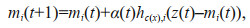 (3)
(3)where t is the sample index of the regression step. The regression is performed recursively for each presentation of a sample of z. The initial values for the model vectors are organized in an orderly fashion along the linear subspace spanned by the two principal eigenvectors of the input data set.
The index c for determining closest pattern is defined by the condition
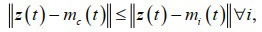 (4)
(4)where||.|| is the distance measure.
Here hc(x), i is called the neighborhood function, which is a decreasing function of the distance between the the ith and cth models on the map grid. It is taken to be the Gaussian
 (5)
(5)where rc is the location of unit c on the map grid and the σ(t) is the neighborhood radius at time t. The learning rate factor α(t) is a decreasing function of time between [0, 1]. It linearly goes from 1 to 0 during the training length.
Various methods have been proposed for determining SOM grid size. SOM analysis is based on finding the smallest Euclidean distance between daily data and SOM patterns, which corresponds to the minimization of the average quantization error (QE). Yuan et al. (2015) defined QE as:
 (6)
(6)where zt is the observed field on each day and mc*is the representative SOM pattern for that day, and N is the number of days. Occurrence frequency of mc*, or f(mc*), is the ratio of the number of samples associated with mc* to N.
Lee and Feldstein (2013) selected the grid size using two criteria on the basis of average pattern correlations between observed daily field and its representative SOM pattern. First, the number of SOM patterns should not be too large; second, SOM patterns should be similar to observed daily fields. We applied this method, which has been used in other studies (Feldstein and Lee, 2014; Yuan et al., 2015). We evaluated quantization errors and average pattern correlations for five grid sizes: 2×4, 3×3, 3×4, 3×5, and 4×4 (Table 1). For each SOM pattern, mean pattern correlation between the daily field and the representative SOM pattern for that day (i.e., the SOM pattern with the smallest Euclidean distance on that day) was calculated. In Table 1, the second column shows the weighted-mean correlation of all SOM patterns; weights were defined by occurrence frequency of the SOM pattern; the third column shows the quantization error. As can be seen, when grid size doubles from 2×4 to 4×4, mean pattern correlation increases from 0.48 to 0.54 and quantization error decreases from 3.89 to 3.67. We performed the SOM analysis with a 3×4 grid because this grid is not too large, its average pattern correlation is relatively high, and its average quantization error is low. We also examined spatial patterns (figures not shown) and occurrence frequencies using different grids and found that the essential features of the main SOM patterns are retained, indicating that the properties of these patterns are insensitive to grid size. We used the software MATLAB and the SOM Toolbox (http://www.cis.hut.fi/projects/somtoolbox/).

|
In addition, EOF analysis was conducted. Although this linear method has some shortness, the leading EOFs can still capture the dominant spatial patterns. The Monte Carlo technique (Overland and Preisendorfer, 1982) was used to test the significance of EOF modes. Composite and correlation methods were also used. Statistical significance was evaluated with Student's t-tests.
3 RESULT 3.1 Intraseasonal variability of the equatorial subsurface temperature continuum 3.1.1 EOF patternsAn EOF analysis was conducted on intraseasonal subsurface temperature anomaly (STA) data from 1993 to 2016; data along equator averaged in from 2°S to 2°N above 300 m were used to extract the linearly dominant ISV patterns (Fig. 2). Monte Carlo test results indicate that the first two EOF modes are significant at the 95% confidence level. Variances are also strongly concentrated in the first two modes.

|
| Fig.2 The first two EOF modes of intraseasonal subsurface temperature anomaly (STA) during 1993–2016 a–b. spatial pattern, EOF1 and EOF2, with the variance fraction showing in the bracket; c–d. corresponding time series of principal component for the first (PC1) and the second (PC2) mode (normalized by the standard deviation); e–f. power spectra of the first and the second time series, with dashed lines denoting 95% confidence level based on Student's t-test. |
The first two modes account for 60% of total STA variance; the first (EOF1) and second (EOF2) modes explain 32% and 28% of the variance, respectively; their spatial patterns are depicted in Fig. 2a & b. Principal components of the leading modes—PC1 for EOF1 and PC2 for EOF2—normalized by their standard deviations are shown in Fig. 2c & d. The EOF1 displays a zonal sandwich pattern along the thermocline with positive loading in the central Pacific and negative loading in the western and eastern Pacific (Fig. 2a). The EOF2 (Fig. 2b) exhibits a seesaw pattern with centers along the thermocline.Spectral analysis suggests that both EOF1 and EOF2 oscillate broadly with periods of 50 to 95 days with peaks at 55 to 60 days and 70 to 80 days, while EOF2 has an additional peak at 90 days (Fig. 2e & f).
3.1.2 SOM patternsTo better resolve spatial variation of intraseasonal variability from nonlinear perspective, we examined SOM patterns extracted from filtered (20–100 days) daily STA data. Figure 3 shows 12 SOM patterns. For each pattern, occurrence frequency—percentage of days over the study period for which a particular pattern is the representative pattern of the day—is shown in the bracket at the top of the figure.

|
| Fig.3 SOM spatial patterns Occurrence frequency of each SOM pattern is shown in bracket. |
By comparing Fig. 3 and Fig. 2, we can see that each EOF is related to a continuum of SOM patterns. To quantify this relationship, we calculated spatial correlations between SOM patterns and the sandwich (EOF1) and seesaw (EOF2) modes (Table 2). If the correlation between a SOM pattern and EOF1 is greater than or equal to the threshold value of 0.7, then we consider that this pattern corresponds to the positive phase of the sandwich mode; if correlation is less than -0.7 then the pattern corresponds to the negative phase of the mode. Similarly, if the correlation between a pattern and EOF2 is greater (less) than or equal to 0.7 (-0.7), then this pattern corresponds to the positive (negative) phase of the seesaw mode.
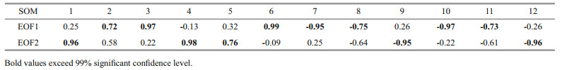
The threshold value was determined following two criteria: 1) the value should be large enough so that each SOM pattern is only associated with one mode, and 2) it should be small enough so that each mode is associated with several patterns. We found three SOM patterns that correspond to the positive phase of the sandwich mode (SOM2, SOM3 and SOM6), four patterns that correspond to the negative phase of the sandwich mode (SOM7, SOM8, SOM10 and SOM11), three patterns that correspond to the positive phase of the seesaw mode (SOM1, SOM4 and SOM5), and two patterns that correspond to the negative phase of the seesaw mode (SOM9 and SOM12).
For each SOM pattern, we generated a corresponding time series by projecting 20–100 days filtered STA data on to the pattern using linear regression; SPC1–12 are the time series for the 12 SOM patterns, and are referred to as the SOM PCs in this paper. Spectral analysis of SOM PCs suggests that SOM patterns oscillate broadly with a period of 50 to 95 days (Fig. 4). Following Yuan et al. (2015) and Johnson and Feldstein (2010), we define the e-folding time scale of a SOM pattern as the time over which autocorrelation decays to 1/e. We found that e-folding time scales of all SOM patterns are between 11 and 12 days (Fig. 5a), and lagged autocorrelations decay to zero over about 15 to 16 days. Principal component time series of the EOFs also yield e-folding time scales of 11 to 12 days (Fig. 5b). The SOM patterns and EOFs have similar e-folding time scales, further proving that SOM patterns oscillate predominantly on the intraseasonal time scale.

|
| Fig.4 Power spectra of regressed time series on SOM patterns (SPC) The dashed line represents a 0.05 significance level. |

|
| Fig.5 Auto-correlation of SOM PCs (a), and EOF PCs (b) |
If we reorder the sequence of the SOM patterns, we can see a wave pattern evolution moving in the positive horizontal axis direction: SOM6 → SOM3 → SOM2 → SOM5 → SOM1 → SOM4 → SOM7 → SOM10 → SOM8 → SOM11 → SOM12 → SOM9, which is consistent with a phase progression of the synthetic sinusoidal pattern. This feature of the continuum SOM patterns together with their oscillation period confirms an eastward propagation in the form of intraseasonal equatorial Kelvin wave. In other words, both seesaw and sandwich patterns from EOF analysis as well as from SOM analysis are one mode in different phases associated with the intraseasonal Kelvin wave.
3.2 Interannual variation of SOM patterns 3.2.1 Correlation analysisIn this section, we examine the relationship of intraseasonal variability and ENSO from a SOM perspective. Because the period of the intraseasonal time scale is about 55 to 90 days, we divided each year into two seasons; spring-summer season is characterized by mean values from April, May, June, July, to August (AMJJA), and autumn-winter season is characterized by mean values from October, November, December to January and February of the following year (ONDJF). For each SOM pattern, seasonal occurrence frequency—percentage of days over the season for which a particular pattern is the representative pattern of the day—between 1993 and 2016 and normalized by standard deviation is shown in Fig. 6 together with the Niño3.4 index. There is clear interannual variation in the occurrence frequencies of SOM patterns, which can also be seen from the lead-lag correlations between the SOM patterns and the Niño3.4 index (Fig. 7). Most patterns are closely correlated to the Niño3.4 index. The Niño3.4 index is defined by the SSTA averaged in (170°W–120°W, 5°S–5°N). The largest positive correlation coefficients are between 0.4 and 0.6 and occur when SOM1, SOM3 and SOM10 lead the Niño3.4 index for 0–1 seasons; correlations are significant at the 99% confidence level. Statistically significant negative correlations occur when SOM5, SOM8 and SOM9 lead Niño3.4 index for 0–1 seasons. These results indicate that occurrence frequencies of SOM1, SOM3 and SOM10 increase (decrease) during El Niño (La Niña) events, while the opposite is true for SOM5, SOM8 and SOM9.

|
| Fig.6 Time series of the seasonal occurrence frequency anomalies and Niño3.4 index Values are normalized by their standard deviation. Two seasons in a year: spring–summer (5 months mean, from April to August) and autumn–winter (5 months mean, from October to February of the following year). |

|
| Fig.7 Lead-lag correlation between the seasonal occurrence frequency for each SOM pattern and Niño3.4 index shown in Fig. 6 |
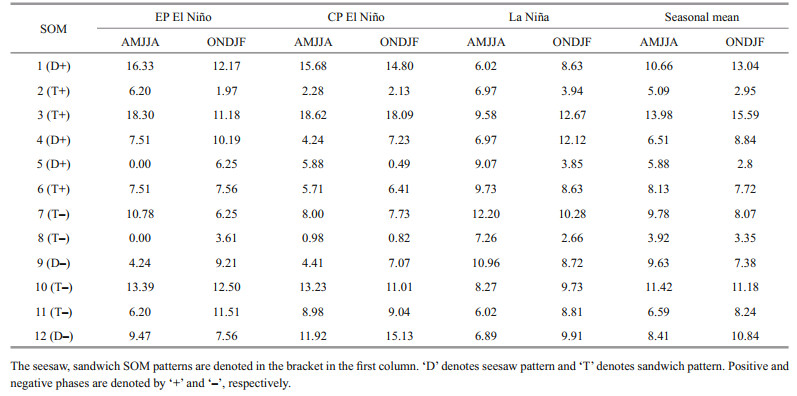
We conducted a composite analysis to investigate whether ENSO influences SOM patterns and their interannual variation. We used the method proposed by Yeh et al. (2009) to identify CP and EP events. An EP El Niño year is defined as the year in which the Niño3 SST index averaged over December, January and February (DJF mean SST anomaly averaged over the Niño3 region, which is located at 150°W–90°W, 5°S–5°N) is above 0.5℃ and greater than the DJF Niño4 SST index (DJF mean SST anomaly averaged over the Niño4 region, which is located at 160°E–150°W, 5°S–5°N). A CP El Niño year is defined as the year in which the DJF Niño4 SST index is above 0.5℃ and greater than the DJF Niño3 SST index. Between 1993 and 2016, there were two EP El Niño events (1997/98 and 2015/16), four CP El Niño events (1994/95, 2002/03, 2004/05 and 2009/10), and eight La Niña events (1995/96, 1998/99, 1999/2000, 2005/06, 2007/08, 2008/09, 2010/11 and 2011/12). Other years were neutral (1993/94, 1996/97, 2000/01, 2001/02, 2003/04, 2006/07, 2012/13, 2013/14 and 2014/15). For each SOM pattern, we calculated its occurrence frequency in EP El Niño, CP El Niño, La Niña and neutral years for the spring-summer and autumn-winter seasons (Table 3).
|
Occurrence frequencies of SOM1, SOM3 and SOM10 generally increase (decrease) during El Niño (La Niña) years; whereas those of SOM5, SOM8 and SOM9 increase (decrease) during La Niña (El Niño) years. For example, occurrence frequency of SOM1 in spring-summer is 10.66% in neutral years, 16.33% (15.68%) in EP (CP) El Niño years, and 6.02% in La Niña years. Occurrence frequency of SOM3 in spring-summer is 13.98% in neutral years, 18.30% (18.62%) in EP (CP) El Niño years, and 9.58% in La Niña years. Occurrence frequency of SOM10 in spring-summer increases to 13.39% (13.23%) in EP (CP) El Niño years from 11.42% in neutral years, and decreases to 8.27% in La Niña years. Occurrence frequencies of SOM5 in spring-summer in EP El Niño, CP El Niño, La Niña and neutral years are 0.0%, 5.88%, 9.07% and 5.88%, respectively; those of SOM8 are 0.0%, 0.98%, 7.26%, and 3.92%, and those of SOM9 are 4.24%, 4.41%, 10.96%, and 9.63%. These results are generally consistent with correlation analysis results although some discrepancies exist because two types of El Niño are included in the composite analysis. Discrepancies are mainly found in autumn-winter of the CP and EP El Niño years. For example, occurrence frequency of SOM1 in autumn-winter increases from 13.04% in neutral years to 14.08% in CP El Niño years, but decreases to 12.17% in EP El Niño years. Similarly, occurrence frequency of SOM9 in autumn-winter decreases from 7.38% in neutral years to 7.07% in CP El Niño years, but increases to 9.21% in EP El Niño years.
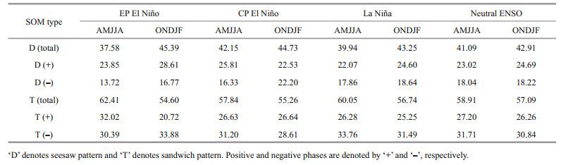
Because most SOM patterns are associated with either the seesaw or sandwich mode, we examined seasonal change in occurrence frequencies of the patterns associated with each mode during different ENSO phases. Positive and negative phases were analyzed together initially. Table 4 shows average occurrence frequencies of SOM patterns associated with positive and negative phases of the seesaw and sandwich modes. As can be seen in Tables 3 & 4, seesaw and sandwich patterns appear in EP El Niño, CP El Niño, La Niña, and neutral years in both seasons.
|
Total occurrence frequencies of the seesaw pattern in spring-summer, which is when ENSO events develop, are 37.58%, 42.15%, 39.94%, and 41.09% in EP El Niño, CP El Niño, La Niña and neutral years, respectively; total occurrence frequencies of the seesaw pattern in autumn-winter, which is when ENSO events are mature, are 45.39%, 44.73%, 43.25%, and 42.91% during EP El Niño, CP El Niño, La Niña and neutral years, respectively. Total occurrence frequencies of the sandwich pattern in spring-summer are 62.41%, 57.84%, 60.05%, and 58.91% in EP El Niño, CP El Niño, La Niña and neutral years; total occurrence frequencies of the sandwich pattern in autumn-winter are 54.60%, 55.26%, 56.74%, and 57.09% in EP El Niño, CP El Niño, La Niña and neutral years. Taking neutral years as a reference, these results indicate that occurrence frequency of the seesaw pattern increases (decreases) during the mature (developing) phase of an ENSO event; occurrence frequency of the sandwich pattern increases considerably during the development of both El Niño and La Niña events, and decreases during the mature phase. In both El Niño and La Niña years, occurrence frequency of the seesaw (sandwich) pattern increases (decreases) from spring-summer to autumn-winter. In other words, the seesaw pattern is more likely to occur during the mature phase of an ENSO event, while the sandwich pattern is more likely to occur during the development of an ENSO event. Meanwhile, occurrence frequency of the sandwich pattern is higher than that of the seesaw pattern.
The positive and negative phases of the seesaw and sandwich patterns were also investigated in detail. Positive seesaw pattern occurs more frequently than negative seesaw pattern, whereas negative sandwich pattern occurs more frequently than positive sandwich pattern. For the seesaw pattern, we found that occurrence frequencies of both positive and negative phases generally increase from spring-summer to autumn-winter; exceptions include the positive phase in CP El Niño years (occurrence frequency of 25.81% in spring-summer and 22.53% in autumn-winter) and the negative phase in neutral years (occurrence frequency of 19.23% in spring-summer and 15.13% in autumn-winter). For the sandwich pattern, occurrence frequency of the positive phase decreases from spring-summer to autumn-winter in EP El Niño, La Niña and neutral years; occurrence frequencies in spring-summer and autumn-winter are similar in CP El Niño years (26.63% in spring-summer, 26.64% in autumn-winter); occurrence frequency of the negative phase increases from spring-summer to autumn-winter in EP El Niño and neutral years, but decreases in CP El Niño and La Niña years.
We used the mean of a SOM PC to quantify the strength of the corresponding SOM pattern. Mean strength was calculated for spring-summer and autumn-winter in EP El Niño, CP El Niño, La Niña, and neutral years. The ISV strength during a certain period is defined by the summary of 12 SOM PCs weighted by its occurrence in the period. Figure 8 shows that ISV oscillations are clearly much stronger in El Niño years than in La Niña and neutral years with some differences between EP and CP El Niño years. The strongest ISV occurs in spring-summer during the developing phase of EP El Niño, and in autumn-winter during the mature phase of CP El Niño. This is in agreement with that argued by Feng et al. (2016).
These results indicate that ENSO has considerable effects on the seasonality of positive and negative seesaw and sandwich patterns.
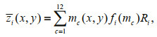
3.2.3 Spatial pattern compositeEach SOM pattern was multiplied by its occurrence frequency, which is weighted by the SOM PC during the composite period, and composite maps were created by summing over all 12 patterns as follows:
 (7)
(7)

|
| Fig.8 Mean strength (no unit) of the intraseasonal variability (ISV) in spring-summer (AMJJA), and autumn-winter (ONDJF) during EP El Niño (EP), CP El Niño (CP), La Niña (LA), and neutral (NE) years |
where zi (x, y) denotes the composite temperature anomaly pattern for period i, mc(x, y) denotes SOM pattern c in Fig. 3, fi(mc) is the average occurrence frequency of mc for period i, and Ri is the average SOM PC in period i. We obtained composite maps for the developing (averaged over AMJJA) and mature phases (averaged over ONDJF) of ENSO events during EP El Niño, CP El Niño and La Niña years (Fig. 9) and compared them with true composite anomaly patterns derived from the original temperature data (Fig. 10).

|
| Fig.9 Composite maps for interannual variability of SOM patterns in different ENSO phases Values in shading are larger than 0.2 (no unit) and exceed 95% confidence level. |

|
| Fig.10 Composite maps for interannual STA in different ENSO phases Values in shading are larger than 0.5 (unit: ℃) and exceed 95% confidence level. |
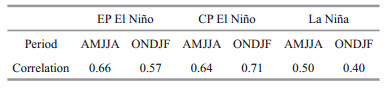
We calculated the correlation coefficients between the composite maps from SOM and the original temperature data. As expected, there is close correlation between the maps and features of ENSO are clearly visible (Table 5). For example, for developing and mature phases of EP El Niño, correlation coefficients are 0.66 and 0.57; for developing and mature phases in CP El Niño, correlation coefficients are 0.64 and 0.71; for developing and mature phases of La Niña, correlation coefficients are 0.50 and 0.40. All correlations are significant at the 99% confidence level. The largest positive loadings for the interannual variability of SOM patterns and the temperature anomaly field are located in the central Pacific during CP El Niño and eastern Pacific during EP El Niño (Figs. 9 & 10), which is consistent with the structural features of the two flavors of El Niño.
|
Except for a high pattern correlation between interannual variation of SOM and the true interannual STA, the dominant mode of intraseasonal STA itself also shows a high similarity with that of the interannual STA. The first and the second EOFs of interannual STA (Fig. 11a & b) are the well-known east-west tilt mode (i.e., seesaw mode) and warm water volume mode, respectively (Meinen and McPhaden, 2000; Clarke, 2010). They represent the different phases of EP El Niño. The correlation between PC1 and Niño3 index reaches as high as 0.95. EOF3 shows a sandwich pattern with positive STA in central Pacific, and negative STA in eastern and western Pacific. This mode is associated with CP El Niño (Kim et al., 2012; Kumar and Hu, 2014). Its time series closely relates to the El Niño Modoki index (Ashok et al., 2007), with correlation between them reaching 0.80. Different from the sandwich pattern shown in Fig. 2a, the central Pacific temperature anomaly stays mainly above the thermocline. Nevertheless, seesaw and sandwich patterns of the interannual STA are still similar with those of the intraseasonal STA. To verify this, we calculated the correlation coefficients between them. Correlation between the seesaw patterns (Figs. 2b & 11a) is 0.40, and that is 0.51 between the sandwich patterns (Figs. 2a & 11c). Both correlations are significant at 99% confidence level.

|
| Fig.11 EOF modes of monthly STA during 1993–2016 a–c. spatial pattern, EOF1, EOF2 and EOF3, with the variance fraction showing in the bracket; d: corresponding time series of principal component for the first (PC1), the second (PC2) and the third (PC3) mode (normalized by the standard deviation). |
Because SOM patterns vary primarily on an intraseasonal time scale we can conclude that interannual variability of subsurface temperature can arise from interannual variability in the occurrence frequencies of intraseasonal SOM patterns. Since the sequence of the SOMs presents the eastward propagation of equatorial intraseasonal Kelvin wave, the changes in occurrence frequency of the seesaw and sandwich SOM patterns between the CP and EP events is due to corresponding change of the intraseasonal Kelvin wave. During CP El Niño, occurrence frequencies of both positive and negative sandwich patterns are higher than those of the seesaw patterns. This implies that Kelvin waves with strongest variations locating at the central equatorial Pacific is more frequent than those with strongest variations locating at the western and eastern equatorial Pacific. Therefore, interannual variation of SOM patterns, hence the propagation features of the Kelvin wave, is a possible reason for increased occurrence of CP El Niño events.
4 CONCLUSIONIn this paper, we examined the intraseasonal variability of equatorial Pacific subsurface temperature and its relationship with ENSO. The SOM is suggested to be useful for the detection of intraseasonal changes in ENSO behavior. Our results show that variation in intraseasonal subsurface temperature is mainly found along the thermocline. Most SOM patterns concentrate zonally in basin-wide seesaw or sandwich structures, which oscillate with a period of about 50 to 90 days, and their sequence displays features of equatorial Kelvin wave. Interannual variation of SOM patterns is closely related to ENSO. During the developing phases of both El Niño and La Niña, occurrence frequency of the sandwich SOM pattern increases, while that of the seesaw SOM pattern decreases. During the mature phase of ENSO events, occurrence frequency of the sandwich pattern decreases, while that of the seesaw patterns increases. The change in occurrence frequency of the seesaw and sandwich SOM patters is due to the change of the intraseasonal Kelvin wave characters. Because of data limitations, we were unable to compare occurrence frequencies of the sandwich and seesaw patterns during years when CP El Niño is inactive. Composite maps of the interannual variability of the SOM patterns and subsurface temperature are closely correlated, implying that interannual variability of ocean temperature can be somewhat reasonably expressed in terms of the interannual variation in occurrence frequency of SOM patterns on intraseasonal time scales. In other words, the interannual variation of the intraseasonal variability may be one of the possible driving mechanisms for ENSO. It is worthy to note that the results obtained in this paper are mainly based on nonlinear SOM analysis from qualitative viewpoint. Quantitative analysis should be conducted to further examine the contribution of intraseasonal variation to ENSO; and numerical models should be used to further examine these issues in future.
5 DATA AVAILABILITY STATEMENTThe datasets generated and/or analyzed during the current study are available from the corresponding author on reasonable request.
6 ACKNOWLEDGMENTThe TAO/TRITON array observation data from the TAO Project Office of NOAA/PMEL. The NOAA_ ERSST_V3b data were provided by the NOAA/OAR/ ESRL PSD, Boulder, Colorado, USA and were obtained from their web site at https://www.esrl.noaa.gov/psd/. We thank Tina Tin, PhD, from Liwen Bianji, Edanz Group China (www.liwenbianji.cn/ac), for editing the English text of a draft of this manuscript.
Ashok H, Yamagata T. 2009. Climate change: the El Niño with a difference. Nature, 461(7263): 481-484.
DOI:10.1038/461481a |
Ashok K, Behera S K, Rao S A, Weng H Y, Yamagata T. 2007. El Niño Modoki and its possible teleconnection. J.Geophys. Res., 112(C11): C11007.
DOI:10.1029/2006JC003798 |
Bjornsson H, Venegas S A. 1997. A manual for EOF and SVD Analyses of Climate Data. Centre for Climate and Global Change Research, McGill University, Montreal.
|
Cai W J, Borlace S, Lengaigne M, Van Rensch P, Collins M, Vecchi G, Timmermann A, Santoso A, McPhaden M J, Wu L X, England M H, Wang G J, Guilyardi E, Jin F F. 2014. Increasing frequency of extreme El Niño events due to greenhouse warming. Nat. Climate Change, 4(2): 111-116.
DOI:10.1038/nclimate2100 |
Choi J, An S I, Kug J S, Yeh S W. 2011. The role of mean state on changes in El Niño's flavor. Climate Dyn., 37(5-6): 1 205-1 215.
DOI:10.1007/s00382-010-0912-1 |
Chung P H, Li T. 2013. Interdecadal Relationship between the mean State and El Niño types. J. Climate, 26(2): 361-379.
DOI:10.1175/JCLI-D-12-00106.1 |
Clarke A J. 2010. Analytical theory for the quasi-steady and lowfrequency equatorial ocean response to wind forcing: the "tilt" and "warm water volume" modes. J. Phys. Oceanogr., 40(1): 121-137.
DOI:10.1175/2009JPO4263.1 |
Feldstein S B, Lee S. 2014. Intraseasonal and interdecadal jet shifts in the northern Hemisphere: the role of warm pool tropical convection and sea ice. J. Climate, 27(17): 6 497-6 518.
DOI:10.1175/JCLI-D-14-00057.1 |
Feng J Q, Wang Q Y, Hu S J, Hu D X. 2016. Intraseasonal variability of the tropical Pacific subsurface temperature in the two flavours of El Niño. Int. J. Climatol., 36(2): 867-884.
DOI:10.1002/joc.4389 |
Feng J, Chen W, Tam C T, Zhou W. 2011. Different impacts of El Niño and El Niño Modoki on China rainfall in the decaying phases. Int. J. Climatol., 31(14): 2 091-2 101.
DOI:10.1002/joc.2217 |
Feng J, Li J P. 2011. Influence of El Niño Modoki on spring rainfall over south China. J. Geophys. Res., 116(D13): D13102.
DOI:10.1029/2010JD015160 |
Gutiérrez J M, Cano R, Cofiño A S, Sordo C. 2005. Analysis and downscaling multi-model seasonal forecasts in Peru using self-organizing maps. Tellus A: Dyn. Meteorol.Oceanogr., 57(3): 435-447.
DOI:10.1111/j.1600-0870.2005.00128.x |
Hendon H H, Liebmann B, Glick J D. 1998. Oceanic Kelvin waves and the Madden-Julian oscillation. J. Atmos. Sci., 55(1): 88-101.
DOI:10.1175/1520-0469(1998)055<0088:OKWATM>2.0.CO;2 |
Hu Z Z, Kumar A, Zhu J S, Peng P T, Huang B H. 2019. On the challenge for ENSO cycle prediction: an example from NCEP Climate Forecast System, version 2. J. Climate, 32(1): 183-194.
DOI:10.1175/JCLI-D-18-0285.1 |
Huang B H, Shin C S, Shukla J, Marx L, Balmaseda M A, Halder S, Dirmeyer P, Kinter Ⅲ J L. 2017. Reforecasting the ENSO events in the past 57 years (1958-2014). J.Climate, 30(19): 7 669-7 693.
DOI:10.1175/JCLI-D-16-0642.1 |
Johnson N C, Feldstein S B, Tremblay B. 2008. The continuum of Northern Hemisphere teleconnection patterns and a description of the NAO shift with the use of selforganizing maps. J. Climate, 21(23): 6 354-6 371.
DOI:10.1175/2008JCLI2380.1 |
Johnson N C, Feldstein S B. 2010. The continuum of North Pacific sea level pressure patterns: intraseasonal, interannual, and interdecadal variability. J. Climate, 23(4): 851-867.
DOI:10.1175/2009JCLI3099.1 |
Johnson N C. 2013. How many ENSO flavors can we distinguish?. J. Climate, 26(13): 4 816-4 827.
DOI:10.1175/JCLI-D-12-00649.1 |
Kessler W S, McPhaden M J, Weickmann K M. 1995. Forcing of intraseasonal Kelvin waves in the equatorial Pacific. J.Geophys. Res., 100(C6): 10 613-10 631.
DOI:10.1029/95JC00382 |
Kim S T, Yu J Y, Kumar A, Wang H. 2012. Examination of the two types of ENSO in the NCEP CFS Model and its extratropical associations. Mon. Wea.. Rev., 140(6): 1 908-1 923.
DOI:10.1175/MWR-D-11-00300.1 |
Kohonen T. 1981. Construction of Similarity Diagrams for Phonemes by a Self-Organizing Algorithm. Helsinki University of Technology, Espoo.
|
Kohonen T. 1995. Self-Organizing Maps. Springer-Verlag, Berlin, Heidelberg. p.106-107.
|
Kohonen T. 2001. Self-Organizing Maps.. 3rd edn. Springer, Berlin, Heidelberg. 501p.
|
Kug J S, Jin F F, An S I. 2009. Two types of El Niño events: cold tongue El Niño and warm pool El Niño. J. Climate, 22(6): 1 499-1 515.
DOI:10.1175/2008JCLI2624.1 |
Kumar A, Hu Z Z. 2014. Interannual and interdecadal variability of ocean temperature along the equatorial Pacific in conjunction with ENSO. Climate Dyn., 42(5-6): 1 243-1 258.
DOI:10.1007/s00382-013-1721-0 |
Kutsuwada K, McPhaden M. 2002. Intraseasonal variations in the upper equatorial Pacific Ocean prior to and during the 1997-98 El Niño. J. Phys. Oceanogr., 32(4): 1 133-1 149.
DOI:10.1175/1520-0485(2002)032<1133:IVITUE>2.0.CO;2 |
L'Heureux M L, Collins D C, Hu Z Z. 2013. Linear trends in sea surface temperature of the tropical Pacific Ocean and implications for the El Niño-southern Oscillation. Climate Dyn., 40(5-6): 1 223-1 236.
DOI:10.1007/s00382-012-1331-2 |
L'Heureux M L, Takahashi K, Watkins A B, Barnston A G, Becker E J, Di Liberto T E, Gamble F, Gottschalck J, Halpert M S, Huang B Y, Mosquera-Vásquez K, Wittenberg A T. 2017. Observing and predicting the 2015/16 El Niño. Bull. Amer. Meteor. Soc, 98(7): 1 363-1 382.
DOI:10.1175/BAMS-D-16-0009.1 |
Lee S, Feldstein S B. 2013. Detecting ozone- and greenhouse gas-driven wind trends with observational data. Science, 339(6119): 563-567.
DOI:10.1126/science.1225154 |
Lee T, McPhaden M J. 2010. Increasing intensity of El Niño in the central-equatorial Pacific. Geophys. Res. Lett., 37(14): L14603.
DOI:10.1029/2010GL044007 |
Leloup J A, Lachkar Z, Boulanger J P, Thiria S. 2007. Detecting decadal changes in ENSO using neural networks. Climate Dyn., 28(2-3): 147-162.
|
Liu Y, Weisberg R H. 2005. Patterns of ocean current variability on the West Florida Shelf using the self-organizing map. J. Geophys. Res., 110: C06003.
DOI:10.1029/2004JC002786 |
Lyu Y L, Li Y L, Tang X H, Wang F, Wang J N. 2018. Contrasting Intraseasonal Variations of the Equatorial Pacific Ocean between the 1997-1998 and 2015-2016 El Niño Events. Geophy. Res. Lett., 45(18): 9 748-9 756.
DOI:10.1029/2018GL078915 |
McPhaden M J, Lee T, McClurg D. 2011. El Niño and its relationship to changing background conditions in the tropical Pacific Ocean. Geophys. Res. Lett., 38(15): L15709.
DOI:10.1029/2011GL048275 |
Meinen C S, McPhaden M J. 2000. Observations of warm water volume changes in the equatorial Pacific and their relationship to El Niño and La Niña. J. Climate, 13(20): 3 551-3 559.
DOI:10.1175/1520-0442(2000)013<3551:OOWWVC>2.0.CO;2 |
Overland J E, Preisendorfer R W. 1982. A significance test for principal components applied to a cyclone climatology. Mon. Wea. Rev., 110(1): 1-4.
DOI:10.1175/1520-0493(1982)110<0001:ASTFPC>2.0.CO;2 |
Ren H L, Wang R, Zhai P M, Ding Y H, Lu B. 2017. Upperocean dynamical features and prediction of the super El Niño in 2015/16: a comparison with the cases in 1982/83 and 1997/98. J. Meteor. Res., 31(2): 278-294.
DOI:10.1007/s13351-017-6194-3 |
Santoso A, Mcphaden M J, Cai W J. 2017. The defining characteristics of ENSO extremes and the strong 2015/2016 El Niño. Rev. Geophy., 55(4): 1 079-1 129.
DOI:10.1002/2017RG000560 |
Smith T M, Reynolds R W, Peterson T C, Lawrimore J. 2008. Improvements to NOAA's historical merged land-ocean surface temperature analysis (1880-2006). J. Climate, 21(10): 2 283-2 296.
DOI:10.1175/2007JCLI2100.1 |
Xue Y, Kumar A. 2017. Evolution of the 2015/16 el Niño and historical perspective since 1979. Sci. China Earth Sci., 60(9): 1 572-1 588.
DOI:10.1007/s11430-016-0106-9 |
Xue Y, Smith T M, Reynolds R W. 2003. Interdecadal changes of 30-Yr SST normals during 1871-2000. J. Climate, 16(10): 1 601-1 612.
|
Yeh S W, Kug J S, Dewitte B, Kwon M H, Kirtman B P, Jin F F. 2009. El Niño in a changing climate. Nature, 461(7263): 511-515.
DOI:10.1038/nature08316 |
Yu J Y, Kao H Y. 2007. Decadal changes of ENSO persistence barrier in SST and ocean heat content indices: 1958-2001. J. Geophys. Res., 112(D13): D13106.
DOI:10.1029/2006JD007654 |
Yuan J C, Tan B K, Feldstein S B, Lee S. 2015. Wintertime North Pacific teleconnection patterns: seasonal and interannual variability. J. Climate, 28(20): 8 247-8 263.
DOI:10.1175/JCLI-D-14-00749.1 |
Zhang C Z. 2001. Intraseasonal perturbations in sea surface temperatures of the equatorial eastern Pacific and their association with the Madden-Julian oscillation. J. Climate, 14(6): 1 309-1 322.
DOI:10.1175/1520-0442(2001)014<1309:IPISST>2.0.CO;2 |
Zhang R H, Zheng F, Zhu J, Wang Z G. 2013. A successful real-time forecast of the 2010-11 La Niña event. Sci. Rep., 3: 1 108.
DOI:10.1038/srep01108 |
Zhu J S, Kumar A, Huang B H, Balmaseda M A, Hu Z Z, Marx L, Kinter Ⅲ J L. 2016. The role of off-equatorial surface temperature anomalies in the 2014 El Niño prediction. Sci. Rep., 6: 19 677.
DOI:10.1038/srep19677 |