 2020, Vol. 38
Institute of Oceanology, Chinese Academy of Sciences
Article Information
- LI Xiang, YUAN Dongliang
- An assessment of the CMIP5 models in simulating the Argo geostrophic meridional transport in the North Pacific Ocean
- Journal of Oceanology and Limnology, 38(5): 1445-1463
- http://dx.doi.org/10.1007/s00343-020-0002-0
Article History
- Received Jan. 3, 2020
- accepted in principle Apr. 14, 2020
- accepted for publication Jul. 22, 2020


2 Center for Ocean Mega-Science, Chinese Academy of Sciences, Qingdao 266071, China;
3 University of Chinese Academy of Sciences, Beijing 100049, China
The latest Coupled Model Intercomparison Project phase 5 (CMIP5) provides hindcast and forecast simulations for the Fifth Assessment Report of the Intergovernmental Panel on Climate Change (Stocker et al., 2014). As an essential component of the global climate system, ocean general circulation plays an important role in redistributing heat, salt, and passive tracers in the world oceans. So far, the simulated transports of the ocean circulation in these coupled models have not been evaluated with observations at the basin scale.
The general ocean circulation theory suggests that the currents of the world oceans are determined by the vertical velocity, like the Ekman pumping, which forces the meridional movement of the water. The vertical velocity in the ocean is very small and difficult to measure directly. In contrast, the meridional velocity can be measured directly and can be used to assess model simulations. The meridional transport can also be used to calculate the zonal transport from the continuity equation. In practice, the large-scale meridional transport is estimated based on geostrophy from temperature and salinity profiles observed in the ocean, since direct current measurements are scarce. The geostrophic currents are estimated based on the thermal wind relation, which usually needs an artificially specified level of no motion in the deep ocean.
To overcome the uncertainty associated with the specification of the level of no motion, several methods have been developed to estimate the absolute geostrophic currents (AGCs) from the density fields of the ocean, such as the β-spiral method (Stommel and Schott, 1977), the box inverse method (Wunsch, 1978), and the P-vector method (Chu, 1995, 2006). The three methods share the same dynamics frame of the thermal wind relation. The β-spiral method uses the second derivatives of the density fields and produces noisy currents. The box inverse method is subject to the uncertainty of a null space of the singular value decomposition. The P-vector method derives the directions of the geostrophic currents from the intersections of the potential density and potential vorticity surfaces (called the P-vector) and uses the triangle formed by the thermal-wind vector and the P-vectors of two depths to determine the magnitudes of the geostrophic currents. It uses only the first derivatives of the density and forms an overdetermined system with the least-square fitting in the vertical. The P-vector and the β-spiral methods are dynamically equivalent under the assumptions of geostrophy, Boussinesq approximation, and conservation of potential density and potential vorticity (Yuan et al., 2014).
However, the transports of the coupled model simulations and the observations cannot be compared with each other directly, because the self-sustained oscillations of the coupled models usually differ from those in reality. For example, biases in the surface wind simulation may lead to biases in the simulated general ocean circulation. An effective approach of assessing the simulated ocean circulation of the coupled models is to examine the dynamics of the system. The Sverdrup balance, which is the first integral of the linear vorticity equation, governs the relation between the mean vertically integrated meridional transport and the mean surface wind stress curl (Sverdrup, 1947). It is the zeroth-order dynamics of the mean wind-driven ocean circulation that can be used to assess the model simulations with observations.
Existing comparisons of the observations with the Sverdrup theory show that the Sverdrup balance is in agreement with the geostrophic currents in the eastern subtropical gyre in the North Atlantic Ocean, but fails to explain the transport of the Gulf Stream and its recirculation (Leetmaa et al., 1977; Wunsch and Roemmich, 1985; Schmitz et al., 1992). In the Pacific Ocean, Meyers (1980) and Hautala et al. (1994) found that the Sverdrup balance is not satisfied in the North Equatorial Countercurrent and in the western subtropical Pacific Ocean. Wunsch (2011) showed that an assimilated dataset using a coarse-resolution ocean model is generally in agreement with the theory. Recently, Argo temperature and salinity profiles provide unprecedented observations of the world oceans with basin-scale synchronicity, base on which the Sverdrup theory has been examined in the North Pacific Ocean and the global ocean (Zhang et al., 2013; Gray and Riser, 2014; Yuan et al., 2014; Yang and Yuan, 2016). Significant non-Sverdrup gyre transports in the tropical and subtropical northwestern Pacific Ocean have been identified by Zhang et al. (2013) and Yuan et al. (2014), the simulations of which in the CMIP5 models have never been examined before.
In this paper, the ability of the CMIP5 models in simulating the Sverdrup and non-Sverdrup gyres of the North Pacific Ocean are assessed using the Argo observations. The heat and salt transports of the nonSverdrup gyre circulation are also estimated, which are compared with the CMIP5 model simulations. The data, the methods, and the Sverdrup theory are described in Section 2. The Sverdrup balance and the meridional volume, heat, and salt transports in the CMIP5 simulations are compared with those of the Argo data in Section 3. In Section 4, the sensitivity of the comparison is discussed and the vorticity balance of one CMIP5 model is analyzed. Conclusions are summarized in Section 5.
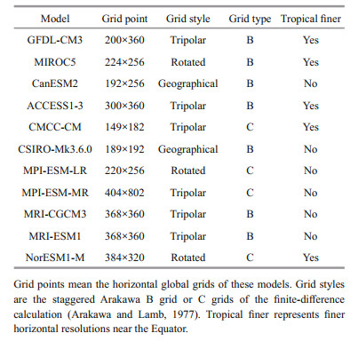
2 DATA AND METHOD 2.1 DataThe CMIP5 multi-model outputs are obtained from the Earth System Grid Federation (ESGF). Among several experiments in the CMIP5 frame, the historical simulations are assessed, which start from the preindustrial periods to the present including both anthropogenic and natural influences. The monthly outputs from 1956 to 2005 of the historical simulations are averaged to form the mean climatological data of the ocean. Eleven global coupled models from different research groups with varying grids and resolutions are selected and analyzed, the detailed information of which is listed in Table 1.
The gridded Argo data are downloaded from the Scripps Institution of Oceanography (SIO) at the website http://www.argo.ucsd.edu/Gridded_fields. html (Roemmich and Gilson, 2009). The horizontal resolution is 1 degree in both zonal and meridional directions. The temperature and salinity profiles are stored in 58 uneven levels in the vertical with the deepest level being 1 975 dbar. The climatological mean data are averaged from January 2004 to December 2018, based on which the P-vector AGCs are calculated. The surface wind vectors of the National Centers for Environmental Prediction (NCEP)-National Center for Atmospheric Research (NCAR) reanalysis 1 product with a horizontal resolution of 2.5° longitude by 2.5° latitude are used to calculate the Sverdrup and Ekman transports. The Large and Pond (1981)'s drag coefficient is used to calculate the wind stress. The time window of the average of the NCEP wind is the same as the Argo data.
2.2 The Sverdrup balanceAssuming the existence of a constant depth with no vertical velocity, the Sverdrup theory gives the balance between vertically integrated meridional velocity and the curl of surface wind stress in the steady state. Nonlinear advection and lateral viscosity are neglected by the theory. Additional terms, like the bottom pressure torque, are also neglected by the theory with the assumption of the existence of a constant depth, beyond which the currents are weak (See Appendix for details).
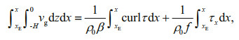
The streamfunction at each longitude (x) is calculated as the meridional volume transport integrated zonally from the eastern boundary (xE) of the basin,
 (1)
(1)where v is the meridional velocity, β is the meridional derivative of Coriolis parameter f, ρ0 the density of sea water under the Boussinesq approximation, τ the surface wind stress, and H the lower limit of vertical integration. Both sides of Eq.1 can be calculated and compared to evaluate the model simulations of the Sverdrup balance.
In practice, another form of the Sverdrup balance is usually used for validation purposes as follows. If the total volume transport is divided into the geostrophic and the Ekman transports, a balance between the geostrophic transport and the Sverdrup minus Ekman transport (S-E transport in abbreviation hereinafter) is obtained,
 (2)
(2)where vg is the geostrophic meridional velocity. H in Eqs.1&2 is roughly 2 000 m in this study (1 975 dbar for the Argo data and the vertical layers closest to 2 000 m for the CMIP5 models).
The comparison between the observations and the CMIP5 simulations with the Sverdrup theory is based on Eq.2. Both Eqs.1&2 are diagnosed for each CMIP5 simulation, using the directly simulated or the geostrophic currents, to examine its agreement with the Sverdrup theory. The discrepancy from the Sverdrup balance is defined as the difference between the left and the right sides of Eqs.1&2, which is called the non-Sverdrup transport in this paper.
2.3 The P-vector absolute geostrophic currentsThe AGCs in this study are calculated using the P-vector method from the density profiles between 1 300 m and 2 000 m. Above 1 300 m, the geostrophic currents are calculated in reference to the velocity at the 1 300 m depth. The use of the 1 300 m depth for the P-vector AGC calculation is to avoid the surface mixing, since the P-vector inversion assumes the conservation of potential vorticity and potential density. The calculated AGCs are not sensitive to the depth range of the P-vector inversion, so long as the depth range is far below the surface mixed layer.
The temperature and salinity data of the CMIP5 simulations are interpolated onto the same 1° longitude by 1° latitude horizontal grid as the Argo data. The vertical coordinates remain unchanged. Then the simulated AGCs are calculated in the same fashion as the Argo AGCs.
2.4 Meridional heat and salt transportsThe observed meridional heat transports (MHT) are estimated from the Argo AGCs and temperature profiles, augmented by the surface Ekman heat transports of the NCEP winds.
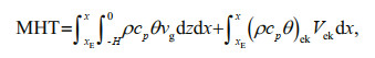 (3)
(3)where ρ, cp, and θ are the sea water density, specific heat capacity, and potential temperature, respectively. The Ekman transport, Vek=-τx/(ρ0f), which is independent of the Ekman layer thickness, is multiplied by the vertically-averaged temperature in the top 50 m of the ocean to represent the surface Ekman heat transport. The vertically averaged temperature in the top 50 m is close to the Ekman layer temperature, so long as the Ekman layer is much shallower than the ocean pycnocline. The small difference of the temperature in the Ekman layer is neglected in this estimate.
Similarly, the meridional salt transports (MST) of the ocean are estimated as the following.
 (4)
(4)where S stands for the salinity of sea water. The MHT and MST of the CMIP5 simulations can also be estimated using the model simulated meridional velocity to replace the geostrophic velocity and the surface Ekman transports. The estimates of MHT and MST using two methods will be compared.
We assume that the geostrophic volume transport is composed of two parts: the S-E and the nonSverdrup transports. A ratio between the S-E transport and the geostrophic transport is calculated at each grid point. A so-called S-E velocity profile is obtained by multiplying the ratio with the geostrophic velocity profile, because the total geostrophic transport contains the parts generated by nonlinear processes (eddy-rectified), which are stipulated by the same stratification through the baroclinic mode functions, with the nonlinear processes considered as forcing terms. Then the S-E MHT and MST are calculated based on the S-E velocity profile and the temperature and salinity profiles. The non-Sverdrup MHT and MST are calculated as the residual of the geostrophic MHT and MST with the S-E MHT and MST subtracted, respectively. In areas where the geostrophic transport is small, the non-Sverdrup transports are simply opposite to the S-E transports. This partition of the non-Sverdrup and the Sverdrup velocity is based on an approximate 1.5-layer system, in which both the linear and nonlinear dynamics are working to transport heat and salt in the same upper layer. More complicated separation of the 3-dimensional Sverdrup and non-Sverdrup transports of heat and salt is beyond the scope of this investigation and is postponed to a separate study.
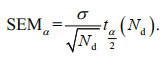
2.5 The standard error of the meanThe standard error of the sample mean (SEM) is estimated as the following.
 (5)
(5)where σ is the standard deviation of the time series, Nd is the degrees of freedom estimated based on the autocorrelation r at one time interval of the sampling (Bretherton et al., 1999).
 (6)
(6)where N is the sample number. The SEM at a given confidence level α is calculated based on the Student's t-distribution test,
 (7)
(7)In this section, the Sverdrup balances in the CMIP5 simulations are first examined and compared with the observations. Then the non-Sverdrup transports of the Argo observations are compared with the CMIP5 simulations to assess the model skills and deficiencies. The MHT and MST of the CMIP5 simulations are then compared with those in the observations to evaluate the deficiencies of the model simulated ocean heat and salt transports in the global climate system.
3.1 The Sverdrup and non-Sverdrup meridional transportsThe comparisons of the CMIP5 simulated and the observed mean geostrophic circulation in the North Pacific Ocean are shown in Fig. 1. These are primarily the Sverdrup gyres forced by the surface wind stress curl. Some differences are noticed between the CMIP5 simulations and the observations. The anti-cyclonic gyres of most of the CMIP5 simulations are stronger by 5 Sv than the observed in the subtropics, whereas the simulated southward transports are weaker in the tropics. The differences of zonally integrated meridional transports between the Argo AGCs and over half of the 11 CMIP5 simulations are as large as or larger than 10 Sv (1 Sv=1×10⁶ m3/s) in the latitudinal range of 10°N–14°N. Considering that the total transport of the tropical gyre is to the north, due to the significant surface Ekman transports (Fig. 2), these comparisons suggest that the CMIP5 models overestimated the tropical and subtropical gyre transports significantly. The effects of these biases of the meridional volume transports on the simulations of climate variability and predictability could be significant. The heat and salt transports comparisons in the next subsection will reveal a glimpse of the effects.

|
| Fig.1 Geostrophic streamfunction of the Argo AGCs in the North Pacific Ocean (a); the CMIP5 simulated geostrophic streamfunctions (b)–(l) minus that of the Argo data (a) Unit is Sv. The intervals of color shadings and contours are 5 Sv and 10 Sv, respectively. |

|
| Fig.2 Ekman streamfunction based on the NCEP winds (a); the CMIP5 simulated Ekman streamfunctions (b)–(l) minus that of the NCEP winds (a) Unit is Sv. The intervals of color shadings and contours are 5 Sv and 10 Sv, respectively |
The S-E streamfunctions based on the NCEP winds and the CMIP5 simulated winds show significant differences in the tropical and subtropical gyres (Fig. 3). The southward S-E transports of all of the 11 CMIP5 simulations are stronger than that of NCEP in the subtropical gyre between 25°N and 35°N. The zonally integrated Ekman transport, which is reciprocal to the Coriolis parameter, is less than 5 Sv north of 25°N (Fig. 2). Therefore, the differences between the CMIP5 models and the NCEP winds north of 25°N are primarily due to biases in the wind stress curl simulations. In the tropics near 10°N, the northward meridional S-E transport is poorly simulated in many of the CMIP5 models. Seven out of 11 CMIP5 models simulate that with the opposite sign. In the subtropical and tropical areas, where large differences of geostrophic meridional transports between the Argo AGCs and the CMIP5 simulations are identified in Fig. 1, the differences of the S-E transport differences are of the same sign with a little larger values (Fig. 3), suggesting that the biases of the ocean circulation in the CMIP5 simulations are primarily due to the wind stress biases. We have also used the wind product of the ERA-Interim reanalysis from the European Centre for Medium-Range Weather Forecasts (ECMWF) to calculate the S-E transport. Nearly the same result has been obtained (figure omitted), suggesting the robustness of the evaluation of the CMIP5 wind stress biases.

|
| Fig.3 Sverdrup minus Ekman (S-E) streamfunction based on the NCEP winds (a); the CMIP5 simulated S-E streamfunctions (b)–(l) minus that of the NCEP winds (a) Unit is Sv. The intervals of color shadings and contours are 5 Sv and 10 Sv, respectively. |
The S-E transports are subtracted from the geostrophic meridional transports to estimate the nonSverdrup gyre circulation in the observations and in the CMIP5 simulations, respectively, which are compared in Fig. 4. The zonally integrated nonSverdrup streamfunction in the Argo data shows values larger than 10 Sv in four zonal bands: two in the tropical gyre (6°N–14°N, 14°N–20°N), one in the subtropical gyre (25°N–35°N), and one in the subpolar gyre (40°N–50°N) (Fig. 4a; also see Yuan et al., 2014). The large values in the subtropical and subpolar areas correspond to the recirculation gyres of the Kuroshio and Oyashio extensions, respectively, suggesting that the non-Sverdrup circulation there is probably induced by nonlinearity of the ocean, like eddies. In the tropical areas, active eddies are also observed in the areas of the non-Sverdrup gyre, suggesting the importance of ocean nonlinearity as well (Yuan et al., 2014).

|
| Fig.4 Non-Sverdrup streamfunctions (Sv) of the Argo AGCs (a), and of the CMIP5 simulations (b)–(l) Unit is Sv. The intervals of color shadings and contours are 2.5 Sv and 5 Sv, respectively. |
The spatial patterns of the non-Sverdrup gyres in the Argo data are not reproduced well by the 11 CMIP5 models, according to the comparison in Fig. 4. All but two (MIROC5 and CSIRO-Mk3.6.0) of the CMIP5 historical simulations fail to simulate the two zonal bands (6°N–14°N, 14°N–20°N) of significant discrepancies from the Sverdrup balance in the tropical North Pacific Ocean. In the subtropical areas of the Kuroshio recirculation and extension, the nonSverdrup streamfunction in most of the CMIP5 simulations is in opposite signs to that in the observations, suggesting deficient dynamics of the CMIP5 models in these areas. In the subpolar gyre, the non-Sverdrup streamfunction in the CMIP5 simulations has the same sign as in the observations, although the magnitude is much smaller.
The magnitudes of the simulated non-Sverdrup streamfunction are much smaller than that in the observations in general. Compared to over 15 Sv of non-Sverdrup meridional transports in the western tropical and subtropical gyres in the Argo data, most models produce non-Sverdrup transports much less than 10 Sv in the North Pacific Ocean. This is understood because these CMIP5 models are of coarse-resolutions and are unable to simulate the oceanic nonlinearity essential for the generation of the non-Sverdrup gyre circulation. The comparisons suggest that these CMIP5 models are deficient in simulating the observed meridional transports in the North Pacific Ocean.
Only two of the CMIP5 models, the MIROC5 and the CSIRO-Mk3.6.0, seem to reproduce the nonSverdrup gyres in the tropical region of 6°N–20°N to some extent. None of them, however, is able to reproduce the non-Sverdrup gyres in the vicinity of the Kuroshio extension, understandably due to lack of eddy activities in the simulations. The dynamics of these models will be further diagnosed in Section 4.3.
The main spatial patterns of the mean Argo geostrophic streamfunction, the streamfunctions based on the Ekman and the Sverdrup theories, and the non-Sverdrup streamfunction based on the differences between the geostrophic and the S-E meridional transports are all found to be above the standard errors of the mean values at the 95% confidence level (Fig. 5, see Section 2.5 for the method). In addition, errors of the Argo geostrophic streamfunction based on the uncertainties of the density profiles are also estimated to be small (Yuan et al., 2014). The CMIP5 simulations are dynamically consistent and are free of observational errors. These facts together suggest that the above comparisons between the CMIP5 simulations and the Argo transports and the diagnosis of the non-Sverdrup streamfunction are all robust. In summary, the biases of the meridional transport simulations in the CMIP5 models come from two sources: the biases in the simulated wind stress curl and the linear dynamic framework that neglect the nonlinear processes essential for the non-Sverdrup gyre circulation.

|
| Fig.5 Standard errors of the mean Argo geostrophic (a), Ekman (b), and the Sverdrup (c) streamfunctions estimated from the standard deviations of the 15 year time series The confidence level is at 95% of the Student's t-test. Intervals for the color shading and contours are 1 Sv and 5 Sv, respectively |
The meridional volume transports carry the heat and salt of the ocean, which are important for global heat and salt balances and climate change. The mean geostrophic MHT and MST of the Argo AGCs are estimated (Fig. 6a & m), showing the dominant equatorward MHT and MST in the subtropical gyre of the North Pacific Ocean of roughly -2.5 PW (1 PW=1×10¹⁵ Watts) and -1.6 ×10⁹kg/s, respectively. The negative sign indicates equatorward. In the tropics, the MHT and MST of the interior gyre are -1.6 PW and -0.8×10⁹ kg/s, respectively. In the subpolar region, the MHT and MST are relatively small.

|
| Fig.6 Geostrophic MHT (a) and MST (m) of the Argo data integrated from the eastern boundary; the CMIP5 simulated MHT (b)–(l) and MST (n)–(x) minus those of the Argo data (a and m, respectively) Units are PW (1015 W) for heat transport and 109 kg/s for salt transport. The intervals of color shadings and contours are 0.3 PW and 0.6 PW, respectively, in (a)–(l), and 0.2×10⁹ kg/s and 0.4×10⁹ kg/s, respectively in (m)–(x). |
Most of the CMIP5 simulations overestimate the geostrophic MHT and MST in the subtropical gyre and underestimate those in the tropical gyre (Fig. 6). In the latitudinal range of 10°N–14°N, the zonally integrated geostrophic MHTs of the tropical gyre of 6 CMIP5 simulations (GFDL-CM3, MIROC5, CMCCCM, MPI-ESM-LR, CSIRO-Mk3.6.0, and MPI ESM-MR) differ from the Argo geostrophic MHT by over 0.9 PW (Fig. 6). The difference is primarily due to the inability of the CMIP5 models to simulate the equatorward geostrophic currents in the western tropical gyre of the North Pacific Ocean.
The Ekman MHT and MST are shown in Fig. 7, which are reminiscent of the Ekman transports (Fig. 2). The Ekman volume, heat and salt transports are large near the equator and decrease with latitude rapidly. The differences of the Ekman transports are due to the biases in the wind simulations in the CMIP5 models. Some of the CMIP5 models (CFDL-CM3, CanESM2, ACCESS1-3, and NorESM1) simulate significantly larger volume, heat, and salt transports than those of the NCEP winds in the tropical gyre south of 10°N because of stronger easterly trade winds simulated in the experiments. The zonally integrated Ekman MHTs of these models (GFDLCM3, CanESM2, ACCESS1-3, and NorESM1) are at least 1.2 PW larger than the observations.

|
| Fig.7 Ekman meridional heat (a) and salt (m) transport of the NCEP-Argo data integrated zonally from the eastern boundary; the CMIP5 simulated Ekman heat (b)–(l) and salt (n)–(x) transports minus those of the NCEP-Argo data (a and m, respectively) Units are PW for heat transport and 109 kg/s for salt transport. The intervals of color shadings and contours are 0.3 and 0.6 PW, respectively, in (a)–(l), and 0.2×10⁹ kg/s and 0.4×10⁹ kg/s, respectively, in (m)–(x). |
The total MHT and MST are estimated by the sum of the geostrophic and the Ekman heat and salt transports (Fig. 8). In the tropical gyre, both the biases in the Ekman MHT and MST and biases in the geostrophic MHT and MST of the CMIP5 simulations contribute to the biases of the total MHT and MST (Fig. 8). In the subtropical gyre, the biases of the total MHT and MST are primarily due to the biases of the geostrophic MHT and MST, since the Ekman MHT and MST are small. At high latitudes, the total MHT and MST biases are small in the North Pacific Ocean.

|
| Fig.8 Total MHT (a) and MST (m) based on the NCEP-Argo data; the CMIP5 simulated MHT (b)–(l) and MST (n)–(x) minus those of the NCEP-Argo data (a and m, respectively) Units are PW for heat transport and ×109 kg/s for salt transport. The intervals of color shadings and contours are 0.3 PW and 0.6 PW, respectively, in (a)–(l), and 0.2×10⁹ kg/s and 0.4×10⁹ kg·s-1, respectively, in (m)–(x). |
The narrow western boundary currents are not resolved by the 1-degree longitude by 1-degree latitude gridded Argo data. Here the total MHT and MST of the interior gyre of the North Pacific Ocean are computed by integrating the Argo transports zonally from the eastern boundary to the vicinity of the WBCs. The sensitivity of the total MHT and MST calculation to the western limits of the integration are examined in Fig. 9. The agreement of the total MHT and MST based on different western limits of the zonal integration suggests that the results are robust for the interior gyres. The largest differences of the MHT and MST between the NCEP-Argo data and the CMIP5 simulations occur in the tropics, where almost all models overestimate the observed transports. In the subtropical gyre, most models overestimate the southward MHT and MST in the observations. The latitudes of the maximum MHT and MST in the CMIP5 simulations are more equatorward than observations (Fig. 9).

|
| Fig.9 Comparisons of total (geostrophic+Ekman) MHT (a–d) and MST (e–h) based on the NCEP-Argo data and the CMIP5 simulations zonally integrated from eastern boundary to 135°E (a, e), 145°E (b, f), 155°E (c, g), 165°E (d, h) Units are PW for heat transport and 109 kg/s for salt transport. Black solid line stands for the NCEP-Argo data. |
To estimate the importance of the non-Sverdrup gyre in transporting heat and salt, we partition the geostrophic volume transport into the S-E transport and the non-Sverdrup transport (see Section 2.4). The MHT and MST of the non-Sverdrup gyre circulation are shown to transport significant amount of heat and salt in the tropical and subtropical gyres based on the Argo data (Fig. 10). In contrast, the four zonal bands of the non-Sverdrup gyres and its associated MHT and MST are poorly simulated by most of the CMIP5 models. The magnitudes of observed non-Sverdrup MHT and MST reach -0.5 PW and -0.45×10⁹ kg/s, respectively, in the tropical gyre, which are several times larger than those of the CMIP5 simulations except in the MIROC5 and CSIRO-Mk3.6.0 models. In general, the non-Sverdrup MHT and MST are comparable in magnitudes with the geostrophic MHT and MST in the observations (Figs. 6a & m, 10a & m) but are significantly smaller than the geostrophic MHT and MST in most of the CMIP5 simulations. The comparisons suggest that the CMIP5 models, which are governed primarily by the Sverdrup balance under linear dynamics, are not able to reproduce the heat and salt transports of the Argo data. It is further suggested that the absence of the non-Sverdrup MHT and MST in the CMIP5 simulations generate significant biases in the coupled climate system model experiments.

|
| Fig.10 Non-Sverdrup geostrophic MHT (a)–(l) and MST (m)–(x) based on the NCEP-Argo data and the CMIP5 simulations Units are PW for heat transport and 109 kg/s for salt transport. The intervals of color shadings and contours are 0.08 PW and 0.16 PW, respectively, in (a)–(l), and 0.15×10⁹ kg/s and 0.3×10⁹ kg/s, respectively, in (m)–(x). |
The sensitivity of the diagnosis of the non-Sverdrup gyre circulation in the Argo data has been discussed in detail in Yuan et al. (2014). The sensitivity of the CMIP5 diagnoses to the lower limit of vertical integration is discussed below.
4.1 The validity of the geostrophic meridional transportsUsing the simulated meridional velocity, the Sverdrup balances in CMIP5 simulations are analyzed based on Eq.1, which show similar biases of the CMIP5 simulations as those based on the geostrophic currents in comparison with the Argo AGCs (Fig. 11 upper panels). Their differences of the upper panels of Fig. 11 from Fig. 4 are the differences due to the geostrophic approximation, which are shown in the lower panels of Fig. 11. The differences of the two are less than 5 Sv in general, suggesting that the geostrophic currents are a reasonable estimate to calculate the volume transports, which also suggest that the use of the Argo AGCs in diagnosing the Sverdrup balance is reasonable. The comparison of the transport calculation using the above two methods was conducted on the eddy-permitting Ocean General Circulation Model for the Earth Simulator (OFES) simulation by Yuan et al. (2014). Their results showed significant non-Sverdrup gyre circulation in the tropics and near the Kuroshio extension, which can be diagnosed by either method with reasonable accuracy. The absence of eddy processes in the coarse-resolution CMIP5 models is likely the reason for the weak nonSverdrup streamfunctions in the CMIP5 simulations.

|
| Fig.11 Argo non-Sverdrup streamfunction above the standard error at the 95% confidence level (a); non-Sverdrup streamfunctions (Sv) of the CMIP5 simulations using Eq.1 (b)–(l); differences between the two estimates of the deviation from the Sverdrup balance (n)–(x), i.e. Fig. 11b-11l minus Fig. 4b–4l Unit is Sv. The intervals of color shadings and contours are 2.5 Sv and 5 Sv, respectively. |
Similarly, the MHT and MST estimations based on the simulated velocity and on the geostrophic approximation are also similar (Fig. 12), suggesting the validity of our analyses. The differences of the MHT and MST due to the geostrophic approximation are generally less than 0.15 PW and 0.1×10⁹ kg/s, respectively, except in the tropics in the model simulations with sizable transport differences, where the differences can be as large as 0.5 PW and 0.3×10⁹ kg/s, respectively (figure omitted). It is worth mentioning that the mean heat and salt transports should also include the covariance between the currents and the temperature and salinity, respectively, in the calculation. We did not estimate the covariance terms due to lack of high-frequency data in the observations and in the model outputs.

|
| Fig.12 Total MHT (a) and MST (m) based on the NCEP-Argo data; the CMIP5 simulated MHT (b)–(l) and MST (n)–(x) using the simulated velocity minus those of the NCEP-Argo data (a and m, respectively) Units are PW for heat transport and 109 kg/s for salt transport. The intervals of color shadings and contours are 0.3 PW and 0.6 PW, respectively, in (a)–(l), and 0.2×10⁹ kg/s and 0.4×10⁹ kg/s, respectively, in (m)–(x). |
The Sverdrup theory assumes that the vertical velocity vanishes at the lower limit of the vertical integration. This depth is difficult to determine in the observations. In the model, the depth at which the vertical velocity is zero or the minimum actually varies with space and time. However, the horizontally varying depth of vertical integration would introduce an additional term of pressure torque, which makes the diagnosis of the Sverdrup balance extremely cumbersome. For simplicity, we diagnosed the Sverdrup balance in the CMIP5 simulations using constant lower limits for sensitivity tests. The results are not sensitive to the specified lower limits between 1 200 m and 3 000 m or between the isopycnal surfaces of 26.7 and 27.2 σ0 (figure omitted). We have also used the depths of the vertical velocity minima as the lower limits of the vertical integration, with the pressure torque term neglected, and the diagnosed Sverdrup balance of the CMIP5 models are essentially the same (figure omitted). Based on the above calculations, we conclude that the diagnoses of the Sverdrup balance in CMIP5 simulations are insensitive to the lower limit of the vertical integration.
4.3 Vorticity balance in the CMIP5 simulationsTo investigate the contribution of each term in the barotropic vorticity equation (Appendix Eq.A2) quantitatively, the vorticity balance of one of the CMIP5 simulations, CSIRO-Mk3.6.0, which reproduces successfully the non-Sverdrup gyres of the observed tropical circulation, is diagnosed. The other CMIP5 model that also reproduces the nonSverdrup gyres of the observed circulation employs time-dependent viscosity (the Smagorinsky-type lateral viscosity), which makes it impossible to estimate the lateral friction term from the monthly output. Therefore, the diagnosis of the vorticity balance is only conducted for the CSIRO-Mk3.6.0 model simulation.
Assuming steady state and neglecting the bottom friction, the vorticity balance of the CSIRO-Mk3.6.0 model simulation is calculated and shown in Fig. 13. The advection term (ADV in Appendix Eq.A2) is large only near the western boundary (See Appendix for the explanation of each term in the vorticity equation). The stretching fw term is more than two orders of magnitude smaller than the advection and the lateral friction terms in the tropical non-Sverdrup gyres. Thus, the lateral friction term (LDF in Appendix Eq.A2) explains the deviation from the Sverdrup balance in the tropical North Pacific in the CSIROMk3.6.0 model simulation.

|
| Fig.13 Distribution of pointwise terms of the vertically integrated vorticity equation diagnosed from the CSIRO-Mk3.6.0 model simulation a. deviation from the Sverdrup balance; b. advection term; c. lateral friction term; d. stretching term. Unit is m2/s. The intervals of color shadings and contours are 0.5 m2/s and 5 m2/s, respectively. |
Lu and Stammer (2004) also used a coarse resolution ocean model to diagnose the vorticity balance, but they found both of the advection and lateral friction play roles in closing the vorticity balance, and the fw term is also significant in hig latitudes. We speculate that the too large lateral viscosity in the CSIRO-Mk3.6.0 model is the main reason for the difference. The large viscosity regarded as a parameterization of the eddy mixing is usually applied in coarse resolution models. Hughes and De Cuevas (2001) used a 0.25° degree eddy-permitting model and found that the advection term is much more important than the lateral friction term in the vorticity balance, implying excessive lateral friction in coarse resolution models.
The non-Sverdrup transport in the tropical Pacific Ocean is found to lead the decadal variability in the North Pacific Ocean (Zhou et al., 2018). The GFDLCM3 simulated meridional transports in Sverdrup balance are found to have no significant correlation with the Pacific Ocean decadal variability. The non Sverdrup transport in the CSIRO Mk3.6.0 is significant in the tropical Pacific Ocean, but it is generated by the extraordinarily large viscosity coefficients and has insignificant correlation with the simulated Pacific decadal oscillation indices also. The effectiveness of the large viscosity parameterization in the coarse resolution climate models needs further validation and study.
As the CMIP6 simulations are released, the nonSverdrup simulations in these higher resolution (e.g. eddy-permitting) models are expected to be improved. The non-linear processes are believed to be the origin of the non-Sverdrup transports, the evaluation of which will be conducted in a future study.
4.4 Sensitivity to the wind productsIn this paper, the biases of the simulated winds of CMIP5 models are assessed based on NCEP winds, which are also used with Argo geostrophic currents to assess the validity of the observed Sverdrup balance. The robustness of the result is indicated by the essential same results obtained using ECMWF winds. The Sverdrup transports are sensitive to the wind products used. For example, the curl and zonal component of the Quikscat winds are found significantly different from those of the reanalysis datasets (NCEP, ERA-Interim, and CCMP) in the tropical Pacific Ocean, the causes of which are still unknown (Zhou et al., 2019). The simulated Sverdrup transports based on the latest Quikscat winds seem to be consistent with the geostrophic meridional transport in the tropical Pacific (Kutsuwada et al. 2019). However, the same wind product reproduces the oceanic recirculation immediate north and south of the Kuroshio extension poorly (not shown). The dynamics of the non-Sverdrup gyre circulation needs further investigation using an eddy-resolving ocean circulation model. The significant difference between the reanalysis and the satellite wind products suggest either significant errors in the reanalyses of the atmospheric circulation or inaccuracies of the satellite wind stress or both.
5 CONCLUSIONIn this study, the geostrophic meridional volume, heat and salt transports of 11 CMIP5 model simulations in the North Pacific Ocean are evaluated based on Argo profiles and NCEP winds. Absolute geostrophic currents are calculated from the density fields of both Argo and the CMIP5 data using the P-vector inverse method.
The results show that the CMIP5 simulations overestimate the tropical and subtropical transports of the Argo data significantly. None of the 11 CMIP5 models simulate the four zonal bands of non-Sverdrup circulation streamfunction in the tropical, subtropical, and the subpolar gyres successfully. The biases are diagnosed to be due to two reasons: the overestimated Sverdrup gyre circulation due to the biases in the wind stress, and the neglect of nonlinear processes essential for the generation of the non-Sverdrup gyre circulation. Analyses show that the above diagnoses are not sensitivity to the lower limits of vertical integration and the use of the geostrophic or directly simulated currents, suggesting that the diagnosed differences are robust.
The CMIP5 models are shown to overestimate the meridional heat and salt transport in the tropical and subtropical gyres. The biases are primarily due to the overestimated Sverdrup gyres in the tropics and subtropics of the North Pacific Ocean. In addition, the non-Sverdrup gyre circulation, which is shown to transport significant heat and salt in the observations, is absent in the CMIP5 simulations. The assessment suggests deficiencies of the CMIP5 model dynamics in simulating the realistic meridional volume, heat and salt transports of the North Pacific Ocean. The biases in the simulated transports suggest that the CMIP5 models are deficient in simulating the mean state of the ocean and the global climate.
The vorticity balance of the CSIRO-Mk3.6.0 model, which simulates the observed non-Sverdrup gyres with some success, is diagnosed using the model output. The analysis suggests that the nonSverdrup circulation in the model is produced by the extraordinarily large lateral friction in the tropical ocean of the model. Further diagnoses need to be conducted to investigate if this kind of parameterization of the sub-grid variability is able to simulate the variability of the meridional transports, which is important for the variability and predictability of the tropical ocean-atmosphere coupled climate system.
The upcoming CMIP6 simulations have much higher resolutions in the ocean models. The comparisons of their simulated meridional transports with the Sverdrup and non-Sverdrup transports based on the Argo profiles are highly expected and are underway at present.
6 DATA AVAILABILITY STATEMENTAll CMIP5 model simulation data are distributed by the Earth System Grid Federation (ESGF) at the website https://esgf-node.llnl.gov/search/cmip5/. The data are open to public without registration.
7 ACKNOWLEDGMENTWe acknowledge the World Climate Research Programme's Working Group on Coupled Modelling, which is responsible for CMIP, and we thank the climate modeling groups for producing and making available their model output.
APPENDIXThe vertically integrated momentum equation is the following.
 (A1)
(A1)Here all the notations are conventional. v is the horizontal velocity vector. 
 (A2)
(A2)β is the meridional derivative of f. ADV and LDF represent the curls of advection (the second term on the left side) and lateral friction terms (last term on the right side) in Eq.A1, respectively. Note that if the z1 and/or z2 vary horizontally, there will be additional terms from the curl of Coriolis term. Also, the curl of pressure gradient will vanish if z1 and z2 are independent of horizontal coordinates. Specially, if z2 is the bottom topography H(x, y), a term of Jacobi of bottom pressure and H(x, y), usually called the bottom pressure torque, will arise.
Arakawa A, Lamb V R. 1977. Computational design of the basic dynamical processes of the UCLA general circulation model. Methods in Computational Physics:Advances in Research and Applications, 17: 173-265.
DOI:10.1016/B978-0-12-460817-7.50009-4 |
Bretherton C S, Widmann M, Dymnikov V P, Wallace J M, Bladé I. 1999. The effective number of spatial degrees of freedom of a time-varying field. J. Climate, 12(7): 1 990-2 009.
DOI:10.1175/1520-0442(1999)012<1990:TENOSD>2.0.CO;2 |
Chu P C. 1995. P-vector method for determining absolute velocity from hydrographic data. Mar. Technol. Soc. J., 29(2): 3-14.
|
Chu P C. 2006. P-Vector Inverse Method. Springer, Berlin. 605p.
|
Gray A R, Riser S C. 2014. A global analysis of Sverdrup balance using absolute geostrophic velocities from Argo. J. Phys. Oceanogr., 44(4): 1 213-1 229..
DOI:10.1175/JPO-D-12-0206.1 |
Hautala S L, Roemmich D H, Schmilz Jr W J. 1994. Is the North Pacific in Sverdrup balance along 24°N? J. Geophys. Res., 99(C8): 16 041-16 052.
DOI:10.1029/94JC01084 |
Hughes C W, De Cuevas B A. 2001. Why western boundary currents in realistic oceans are inviscid:a link between form stress and bottom pressure torques. J. Phys.Oceanogr., 31(10): 2 871-2 885.
DOI:10.1175/1520-0485(2001)031<2871:WWBCIR>2.0.CO;2 |
Kutsuwada K, Kakiuchi A, Sasai Y, Sasaki H, Uehara K, Tajima R. 2019. Wind-driven North Pacific Tropical Gyre using high-resolution simulation outputs. J. Oceanogr., 75: 81-93.
DOI:10.1007/s10872-018-0487-8 |
Large W G, Pond S. 1981. Open ocean momentum flux measurements in moderate to strong winds. J. Phys.Oceanogr., 11(3): 324-336.
DOI:10.1175/1520-0485(1981)011<0324:OOMFMI>2.0.CO;2 |
Leetmaa A, Niiler P, Stommel H. 1977. Does the Sverdrup relation account for the mid-Atlantic circulation? J. Mar.Res., 35: 1-10.
|
Lu Y Y, Stammer D. 2004. Vorticity balance in coarseresolution global ocean simulations. J. Phys. Oceanogr., 34(3): 605-622.
DOI:10.1175/2504.1 |
Meyers G. 1980. Do Sverdrup transports account for the Pacific North Equatorial Countercurrent? J. Geophys.Res., 85(C2): 1 073-1 075.
DOI:10.1029/JC085iC02p01073 |
Roemmich D, Gilson J. 2009. The 2004-2008 mean and annual cycle of temperature, salinity, and steric height in the global ocean from the Argo Program. Prog. Oceanogr., 82(2): 81-100.
|
Schmitz Jr W J, Thompson J D, Luyten J R. 1992. The Sverdrup circulation for the Atlantic along 24°N. J. Geophys. Res., 97(C5): 7 251-7 256.
DOI:10.1029/92JC00417 |
Stocker T F, Qin D, Plattner G K. 2014. Technical summary.In:Climate Change 2013:the Physical Science Basis.Working Group I Contribution to the Fifth Assessment Report of the Intergovernmental Panel on Climate Change. Cambridge University Press, Cambridge, p.33-115.
DOI:10.1017/CBO9781107415324.005 |
Stommel H, Schott F. 1977. The beta spiral and the determination of the absolute velocity field from hydrographic station data. Deep Sea Res., 24(3): 325-329.
DOI:10.1016/0146-6291(77)93000-4 |
Sverdrup H U. 1947. Wind-driven currents in a Baroclinic ocean; with application to the equatorial currents of the eastern Pacific. Proc. Natl. Acad. Sci. USA, 33(11): 318-326.
DOI:10.1073/pnas.33.11.318 |
Wunsch C, Roemmich D. 1985. Is the north Atlantic in Sverdrup balance? J. Phys. Oceanogr., 15(12): 1 876-1 880.
DOI:10.1175/1520-0485(1985)015<1876:ITNAIS>2.0.CO;2 |
Wunsch C. 1978. The North Atlantic general circulation west of 50°W determined by inverse methods. Rev. Geophys., 16(4): 583-620.
DOI:10.1029/RG016i004p00583 |
Wunsch C. 2011. The decadal mean ocean circulation and Sverdrup balance. J. Mar. Res., 69(2-3): 417-434.
|
Yang L N, Yuan D L. 2016. Absolute geostrophic currents in global tropical oceans. Chin. J. Oceanol. Limnol., 34(6): 1 383-1 393.
DOI:10.1007/s00343-016-5092-3 |
Yuan D L, Zhang Z C, Chu P C, Dewar W K. 2014. Geostrophic circulation in the tropical north pacific ocean based on Argo profiles. J. Phys. Oceanogr., 44(2): 558-575.
DOI:10.1175/JPO-D-12-0230.1 |
Zhang Z C, Yuan D L, Chu P C. 2013. Geostrophic meridional transport in tropical northwest Pacific based on Argo profiles. Chin. J. Oceanol. Limnol., 31(3): 656-664.
DOI:10.1007/s00343-013-2169-0 |
Zhou H, Liu X Q, Xu P. 2019. Sensitivity of Sverdrup transport to surface wind products over the tropical North Pacific Ocean. Ocean Dyn., 69(5): 529-542.
DOI:10.1007/s10236-019-01260-8 |
Zhou H, Yuan D L, Yang L N, Li X, Dewar W. 2018. Decadal variability of the meridional geostrophic transport in the upper tropical North Pacific Ocean. J. Climate, 31(15): 5 891-5 910.
DOI:10.1175/JCLI-D-17-0639.1 |