 2020, Vol. 38
Institute of Oceanology, Chinese Academy of Sciences
Article Information
- DAI Jun, WANG Huizan, ZHANG Weimin, AN Yuzhu, ZHANG Ren
- Observed spatiotemporal variation of three-dimensional structure and heat/salt transport of anticyclonic mesoscale eddy in Northwest Pacific
- Journal of Oceanology and Limnology, 38(6): 1654-1675
- http://dx.doi.org/10.1007/s00343-019-9148-z
Article History
- Received Jun. 7, 2019
- accepted in principle Jul. 29, 2019
- accepted for publication Sep. 27, 2019


2 P. O. Box 5111, Beijing 100094, China
Mesoscale eddies are ubiquitous in oceans worldwide (Wang et al., 2003; Chelton et al., 2011; Nan et al., 2011; Zhang et al., 2017), and play a major role in the dynamic conditions, mass or heat transport, potential fishing zones, water mass modification, marine biology, and air-sea interactions of the ocean (Kusakabe et al., 2002; Ma et al., 2016).
Mesoscale eddies in oceans have been extensively studied worldwide over the past 40 years using in-situ measurements, satellite observations, and model simulations (Dong et al., 2017; Li et al., 2019). Sea level anomaly (SLA) maps from satellite altimeters are highly useful for identifying mesoscale eddies. Previous studies based on satellite observations often focused on the statistical characteristics of mesoscale eddies, such as their numbers, amplitudes, rotational speeds, shapes, trajectories, lifetimes, propagation distances, and geographical distributions (Chelton et al., 2011). However, the satellite observations can only reflect the features of the sea surface. Model simulation can determine the structure of mesoscale eddies. For example, Lin et al. (2015) studied the three-dimensional properties of mesoscale eddies in South China Sea based on the output of the eddyresolving model. However, model results may contain some uncertainties and errors. In-situ data from shipboard observations, moorings, and gliders are mainly used to study the structure of an individual mesoscale eddy. For example, Swart et al. (2008) used shipboard observations to study an eddy that formed in the Southern Ocean, which carried anomalous heat and salt content for 1.5° of latitude during its lifetime. Shu et al. (2016) presented the detailed structure of an anticyclonic eddy during spring 2015 in the northern South China Sea by using high-resolution in-situ data from gliders, while Garreau et al. (2018) monitored the vertical structure of a particular anticyclonic eddy in the Algerian Basin from its creation to its dissipation using highresolution (Seasoar) hydrological transects, CTD casts, and LADCP measurements. Qiu et al. (2018) investigated the three-dimensional structure of a warm eddy using three Chinese underwater gliders in the northern South China Sea, while Busireddy et al. (2018) studied the subsurface thermohaline structures of an unusual anticyclonic eddy in the northern Bay of Bengal using two Indian moored buoys. Furey et al. (2018) analyzed a new set of deep float trajectory data collected at depths of 1 500 and 2 500 m to study deep eddies in the Gulf of Mexico, and Steinberg et al. (2019) repeatedly surveyed a California undercurrent eddy (Cuddy) for over three months using multiple sea gliders. Shu et al. (2019) conducted field observations using 12 gliders and 62 expendable probes to investigate the three-dimensional structure and temporal evolution of an anticyclonic eddy in the northern South China Sea during summer 2017.
Argo has been expanded to become a major component of the ocean observation system, and its observations are mainly used to study the composite structure of mesoscale eddies. For example, Chaigneau et al. (2011) reconstructed the mean three-dimensional eddy structure in the eastern South Pacific Ocean by conducting composite analysis using altimetry data and Argo profiling floats, and Yang et al. (2013) explored three-dimensional eddy structures using composite eddy images constructed by surfacing Argo data into altimeter-detected eddy areas in the northwestern subtropical Pacific Ocean. Using collocated altimetry sea surface height anomalies and Argo profiles within detected eddies, Sun et al. (2017) investigated structures of temperature, salinity, potential density in the Kuroshio extension region under the influences of oceanic eddies. Dong et al. (2017) investigated the three-dimensional structures and transport of mesoscale eddies in the northwestern Pacific Ocean using both satellite and Argo float data, while Keppler et al. (2018) detected mesoscale eddies in the southwest tropical Pacific Ocean using satellite altimetry data and then colocalized the detected eddies with Argo floats to determine their vertical structure and their effects on water masses.
The Argo array of 3 200 floats is distributed over the global oceans with an average spacing of 3°, and the individual floats will cycle to a depth of 2 000 m depth every 10 days. Often, we have only a limited number of profiles for an individual eddy, which is very sparse for eddy case studies. In other words, limited by observational method, few targeted observations have been made for individual mesoscale eddies, particularly of their three-dimensional structures and variations. Owing to the "Response of the Indo-Pacific Oceans to global warming and their role in climate change" project (Xie, 2013) funded by the National Key Basic Research (973) Program of China, an eddy-resolving Argo array with 17 rapidsampling Argo floats was deployed in an anticyclonic eddy. Previous studies using these Argo floats have mainly focused on the mode-water in this eddy or sub-thermocline eddies. For example, Zhang et al. (2015) observed two sub-thermocline eddies (STEs), while Xu et al. (2016) observed the effects of a mesoscale eddy on mode-water subduction and transport in the North Pacific. In this study, the spatiotemporal variations of the three-dimensional structure and heat/salt transport of this anticyclonic mesoscale eddy are studied using the 17 Argo floats and an SLA dataset.
2 DATA AND METHOD 2.1 Argo dataDuring the Pacific Mode-Water Ventilation Experiment cruise, 17 Argo-profiling floats with enhanced daily sampling were deployed in an anticyclonic eddy in the western Pacific Ocean (135°E–155°E, 26°N–42°N) in late March, 2014, which observed the anticyclonic eddy from April to September 2014. The Argo floats drift at a parking level of 500 m and record the temperature/salinity (T/S), dissolved oxygen concentration (DO), and pressure (P) from a depth of 1 000 m to the sea's surface with a sampling interval of 24 h. The vertical resolution of the profiles is approximately 2 m above and 10 m below 600 m (Zhang et al., 2015). All of the data collected by these Argo floats were downloaded from China Argo Real-time Data Center (http://www.argo.org.cn).
2.2 Satellite altimeter dataThe daily SLA data with quality control were provided by the CMEMS (Copernicus Marine Environment Monitoring Service) (http://marine.copernicus.eu/). The global ocean gridded L4 Sea Surface Heights and Derived Variables Reprocessed Product was used to identify the anticyclonic mesoscale eddy here, which was gridded on a grid of 0.25°×0.25° with a time interval of one day. This product is processed by the SL-TAC multimission altimeter data processing system. It processes data from all altimeter missions: Jason-3, Sentinel-3A, HY-2A, Saral/AltiKa, Cryosat-2, Jason-2, Jason-1, T/P, ENVISAT, GFO, and ERS1/2. The SLA data are computed with an optimal and centered computation time window (6 weeks before and after the date).
2.3 CARS2009 climatology dataThe climatology data were provided by CSIRO Atlas of Regional Sea 2009 (CARS2009) (http://www.marine.csiro.au/-dunn/cars2009/), which was gridded on a grid of 0.5°×0.5°. Compared with other climatology data, CARS2009 is more suitable for western boundary region (Yang et al., 2013). The climatology data was based on all available marine observation data and automatic buoy profile data in history, and had passed the quality control. The formula for calculating the climate state of CARS2009 on a given day is as follows:
 (1)
(1)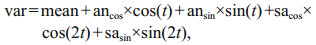 (2)
(2)where "day" is the day number of the year, "var" is the temperature (or salinity) climatology, and "mean", "ancos", "ansin", "sacos", "sasin" are global three-dimensional fields provided by CARS2009. The three dimensional structure of the temperature or salinity climatology of a certain day can be obtained through Eqs.1 and 2. The temperature or salinity climatology of a certain profile position on that day can be directly interpolated from the three dimensional structure of climatology.
2.4 Eddy identification and tracking methodThe eddy identification followed here mainly refers to the method of Ni (2014). The identification method was modified from the two similar methods presented by Chaigneau et al. (2009) and Chelton et al. (2011). The method is an SLA contour-based method, and it has great advantages over the commonly used Okubo-Weiss method in terms of correctness and accuracy (Souza et al., 2011). By comparing three automatic detection algorithms in the South Atlantic, Souza et al. (2011) showed that the geometric criterion used in this study exhibits a better performance, mainly in terms of the eddy detection number, their lifetimes, and propagation velocities. This method was mainly conducted to determine the center and boundary. Here, we considered the center of the eddy to be located at the geometric center of the innermost closed contour of the sea surface height. The contour of the sea level that contains the center of the eddy, which is located at the outermost side, was considered the edge. Once the center and edge of an eddy are identified, its parameters (amplitude, type, and radius) can be computed.
The eddy was tracked following the method used by Chaigneau et al. (2008). For each eddy (e1) identified at a certain position at time t1 and for each eddy (e2) identified at the next position at time t2 and rotating in the same direction than e1, the nondimensional number Se1, e2 can be defined as:
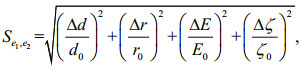 (3)
(3)where Δd, Δr, ΔE, and Δζ, are respectively the distance difference, radius difference, eddy kinetic energy difference, and vorticity difference between e1 and e2, respectively. The algorithm selects the eddy pair (e1, e2) that minimize Se1, e2 and considers this pair to be the same eddy that is tracked from t1 to t2 (Chaigneau et al., 2008). The standard distance d0, radius r0, eddy kinetic energy E0, and vorticity ζ0 are 100 km, 100 km, 100 cm2/s2, and 10-6/s, respectively. To prevent the two different tracks from continuing end-to-end, Δd must be smaller than the search radius, which generally approximates the product of the local average flow velocity and temporal resolution of the data (Nencioli et al., 2010). The method allows to considerably reduce the number of "false" detected eddies (Chaigneau et al., 2008). In addition, this method can also avoid trajectory interruption and has wider application range (Chen et al., 2011).
Figure 1 shows the specific process of eddy identification and tracking.

|
| Fig.1 Eddy identification and tracking flow-chart |
Assuming that the same type of eddy in a certain area has a similar structure, the three-dimensional structure of the composite eddy can be constructed by combining altimeter SLA data, Argo profile data and climatology data (Chaigneau et al., 2011; Yang et al., 2013). The specific method is firstly to use SLA data to detect and track the eddy, then matches the Argo profile with the identified eddy, and obtain the structure of the composite eddy through DIVA interpolation and other process. Based on the method reported by Chaigneau et al. (2011), the Argo profiles are selected according to the following conditions: (1) the shallowest data in the Argo profile is located between the sea surface and 10×104 Pa, and the deepest data point is located below 1 000×104 Pa; (2) the depth interval between two consecutive data does not exceed a given range; (3) there are at least 30 valid data points in each Argo profile.
The temperature, salinity, and dissolved oxygen concentration data of the screened Argo profile were divided into 501 layers by 2×10⁴ Pa from the sea's surface to 1 000×104 Pa in the vertical direction. We took 1 000 dbar isobaric surface as the reference plane here (Chaigneau et al., 2011), and calculated the dynamic height D. The dynamic height D is computed as follows:
 (4)
(4)α is the specific volume, P0 is the reference plane. The temperature anomaly T', salinity anomaly S', and dynamic height anomaly D' can be obtained by subtracting CARS2009 climatology of the same latitude and longitude on the same day from the Argo profile.
In this study, one unit consists of 20 days, and the profiles from April to September 2014 are divided into the following seven periods for composition: April 1–April 21, April 21–May 11, May 11–May 31, May 31–June 20, June 20–July 10, July 10–July 30, and July 30–Sept 2. The final period is 34 days. Figure 2 presents a scatter diagram of the profiles for each period.

|
| Fig.2 Scatter diagrams of the Argo profile position in the seven periods |
DIVA (Troupin et al., 2012; Song et al., 2019) is a multidimensional variational interpolation method and an implementation of the variational inverse method (VIM). The method uses the minimum cost function to interpolate the observed values into an orthogonal grid and aims to derive a continuous field close to the observed values. The cost function is:
 (5)
(5)where dj is the value measured at position (xj, yj), uj represents the weight, and ‖φ‖ is as follows:
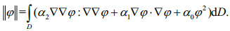 (6)
(6)The smoothness constraint term 
 (7)
(7)where α0 represents the coefficient of a continuous field, α1 is the gradient, and α2 is the rate of change. The method decouples naturally disconnected areas based on topography and topology. It is very useful in oceanography because in fact the disconnected water masses often have different physical properties. However, it is difficult for optimal interpolation to decouple water masses separated by land and maintain at the same time a spatially smooth field over the ocean (Barth et al., 2014). Compared with the twodimensional analysis (horizontal analysis only), the improvement of the three-dimensional analysis (longitude, latitude and time) is that the RMS error decreases relatively much after including advection constraints (stable in the two-dimensional case and varying with time in the three-dimensional case).
In the previous section, Argo data were interpolated into 511 standard layers. The DIVA method first calculates the mean and standard deviation of each standard layer's temperature, salinity, and oxygen field. The median filter is then applied to the result and the difference between the mean and observed values is calculated. If the absolute value of the difference is three times higher than the standard deviation (Song et al., 2019), the profile will be removed and regarded suspicious data, otherwise, it will be retained as trusted data. The data collected from April to September were divided into seven periods. The DIVA function is used to merge the scattered data from each period's profiles to obtain the temperature, salinity, and oxygen field.
3 RESULT AND ANALYSIS 3.1 Eddy trajectoryWe use the SLA data from CMEMS from November 1, 2013 to September 30, 2014 to do the identification and tracking. The result showed the eddy was originated at (154.37°E, 31.13°N), died out at (140.36°E, 28.51°N), translating westward for 269 days from December 6, 2013 to August 31, 2014. The trajectory of the mesoscale eddy is shown in Fig. 3. According to the trajectory map and the depth curve (Fig. 4b), we find that the eddy firstly translating over a relatively flat area about 6 000 m deep, then over the Izu-Ogasawara Trench, after that the eddy began to cross the Izu Ridge. It moved westward 14° of longitude and moves approximately 3° of latitude to the south during its lifetime. This result is consistent with the Chelton's global eddy-tracking dataset (http://wombat.coas.oregonstate.edu/eddies/index.html).

|
| Fig.3 Trajectory of the eddy center The red line represents the trajectory. The yellow point represents the location where eddy generated. The yellow star represents the location where 17 Argo floats were deployed on Apr. 1. Three yellow lines represent the initiation, maturity, and termination phase. |

|
| Fig.4 Variations of the eddy radius (a), depth (b), amplitude (c), and eddy kinetic energy (d) during its lifetime In a, the ⅰ, ⅱ, ⅲ represent the initiation, maturity, and termination phase, respectively. |
The mesoscale eddy's radius, depth, amplitude, eddy kinetic energy variation over its lifetime are shown in Fig. 4. Dong et al. (2012) and Lin et al. (2013) noted that the lifetime of the eddy could be divided into three phases, i.e., the generation, maturity, and termination phases. To describe the structure characteristics in different phases more clearly, we define the first period from April 1 to 21 as the initiation phase of the mesoscale eddy, the fifth period from June 20 to July 10 as the maturity phase, and the final period from July 30 to September 2 as the termination phase. In this study, our Argo floats were deployed from the April 1, and the float did not catch the generation of the eddy, so we rename the first 20- day period from April 1 to April 21 "initiation phase". In addition, our analysis in the paper focus on the date from April 1 to Sept. 2 supported by the 17 Argo floats.
The eddy had an average radius of 91.5 km in its lifetime. The value is larger than the Rossby radius of deformation of 49.76 km computed in the study region (Chelton et al., 1998). The radius maximum reached 170 km in the maturity phase. The eddy radius experienced a great enhance in the maturity phase, and had a rapid drop after entering the termination phase. We will discuss and explain it in detail below from the view of eddy's adjustments to topography. The amplitude and eddy kinetic energy had a similar variation trend with the eddy radius.
In Fig. 4, we find the eddy radius greatly enhanced when entering the maturity phase (phase ⅱ), we considered the conservation of PV can interpret the phenomenon. The conservation of PV is as follows:
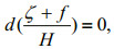 (8)
(8)where H represents depth, and ζ, f represent the relative vorticity, planetary vorticity, respectively. When eddy continued to propagate westward, the depth became smaller, meaning that H was getting smaller. The latitude can be considered a constant during this period, indicating that the planetary vorticity f=2Ωsinφ is also a constant. According to equation, the planetary vorticity ζ tends to decrease, which means a strength for the anticyclonic eddy. Therefore, we consider this reason led to the great enhance of radius in maturity phase.
The experiments of Kamenkovich et al. (1996) and Beismann et al. (1999) also supported the rapid increase in radius. Kamenkovich et al. (1996) did a series of numerical experiments with a two-layer primitive equation model, and found that eddies crossing the ridge show an intensification before the eddy center encounters the ridge, expressed a deepening of the thermocline depth and a heightening of the sea surface elevation. The effect is large enough (O(10)cm for the sea surface elevation) that to be observable in the real ocean with altimeter data. Beismann et al. (1999) also found the same effect that eddies show an intensification by the deflection of the layer interface when approaching the upslope. In this study, when the eddy was over the trench, eddy's western edge had arrived the eastern slope of the Izu Ridge at that time, and the eddy center would encounter the ridge soon. From Fig. 4c, we also observed the amplitude had a great enhance. Therefore, we speculate that the eddy radius's greatly enhancement is also relative to this kind intensification.
When the eddy encountered the Izu Ridge, the eddy translated northwestward along the upslope. Then it continued westward until encountered a higher region of Izu Ridge. After July 30, the radius decreased rapidly. Beismann et al. (1999) found that sufficient topographic heights and strong slopes can even block the eddies and force them toward a pure meridional movement. Therefore, we thought that the rapid drop of radius was mainly because the eddy was blocked by the high ridge and began to dissipate.
3.3 Temperature field structureBefore discussing the eddy's three-dimensional structure, it is necessary to introduce the main water masses properties in the study area. The water in the upper layer is the North Pacific surface water, showing high temperature and low salt characteristics. Based on the Argo profile outside the eddy and CARS2009 climatology, the θ-S diagram (Fig. 5) of the study area shows an obviously reversed "S" shape, with two salinity extrema featuring two water masses: the subsurface high-salinity North Pacific Tropical Water (NPTW) and the low-salinity North Pacific Intermediate Water (NPIW). NPTW's average salinity is up to 34.87, potential density is about 24.4 kg/m3 NPIW's average salinity is from 34.2 to 35, and potential density is about 26.72 kg/m3. Between the subsurface layer and the intermediate layer, the North Pacific Subtropical Mode Water (STMW)'s temperature is 16.0–21.5℃, salinity is 34.65–34.95, and potential density is 24.2–25.6 kg/m3 (Dong et al., 2017; Ni, 2014). Although the Lighter Central Mode Water (L-CMW) (θ=10.0–16.0℃, S=34.44–34.65, σθ=25.4–26.3 kg/m3) are reported to be generated mainly at the region 33°N–39°N, the θ-S diagram in our study area also revealed clear signal of the L-CMW. The part of the reason might be that the formation region of L-CMW shifts southeastward crossing the KE axis (Oka et al., 2011). The yellow dashed line shows the eddy's origin surrounding feature. From initiation to termination phase, the curves are basically the same and salinity minimum is getting larger. It is consistent with Dong et al. (2017) that NPIW becomes saltier as spreading westward, which is likely caused by intensive mixing.

|
| Fig.5 The θ-S diagram of the study area in different phases The θ-S diagram of initiation, maturity, and termination phase were based on the Argo profile outside the eddy. The diagram of origin was based on the CARS2009 climatology. |
Previously, the Argo data were interpolated to 511 standard layers. Based on the DIVA function described above, the temperature distribution of each depth layer was plotted using 20-day Argo composite data. Figure 6 presents an example of a 20-day horizontal section from May 11 to May 31, with a depth ranging from 100 to 1 000 m. The center of the composite eddy was located at Δx=0; Δy=0. The 100-m layer does not clearly reflect the eddy structure. From 200 to 1 000 m, the highest temperature is clearly located at the center, and the eddy structure is distinct. Combined with the Sections 3.3, 3.4, 3.5, the influence depth of the eddy reaches 1 000 m.

|
| Fig.6 Horizontal section of temperature at different depths from May 11 to May 31 |
Temperature slice of each layer corresponding to the initiation phase, maturity and termination phase are presented in Fig. 7. The temperature field of each layer were computed by the DIVA interpolation method. The isotherm was distributed disorderly at 100 m, and was most densely distributed between 400 and 500 m. During the initiation phase, the closed isotherm distribution in the upper layers is sparse, and the isotherm is closer to the center during the maturity phase.

|
| Fig.7 Temperature slices for the initiation (a), maturity (b), and termination (c) phases |
To obtain the temperature anomaly Δθ, the CARS2009 (CSIRO ATLAS OF REGIONAL SEAS) climatology data, which were developed by CSIRO Marine and Atmospheric Research, were linearly interpolated to each Argo profile of the mesoscale eddy, and the vertical profiles of the temperature anomalies Δθ was obtained by subtracting the interpolated data from the composite Argo profile data.
Figure 8 shows that there is a distinct temperature anomaly core at a depth from 400 to 600 m. The temperature anomaly Δθ gradually grew over time; the maximum in the termination phase is larger than +3℃. The average temperature anomaly core Δθ in the eddy's lifetime was +2.5℃. The depth of the temperature anomaly core remained from 400 to 600 m during the lifetime of the eddy, and the temperature gradient around the core was largest during the termination phase.

|
| Fig.8 Profile of temperature anomaly in the zonal direction during the three phases |
To explore the influence of the mesoscale eddy on the vertical distribution of temperature, the difference between the Argo profile and background field temperature in the center of this eddy during each period is plotted in Fig. 9. The thin lines with different colors represent Δθ in the seven periods, the red dashed line represents the average Δθ during the lifetime of the eddy. From the surface to 500 m, Δθ gradually increased with depth to a maximum value of 1.7℃ approximately from 400 to 600 m, corresponding to the temperature anomaly core of the eddy. The temperature anomaly core all located between 25.5–26 kg/m3 of potential density in three phases. We inferred that the water trapped by eddy was below the NPTW (about 24.4 kg/m3) and above the NPIW (about 26.72 kg/m3). From 500 to 800 m, Δθ decreased during each period, indicating that the strength of the eddy's structure weakened. The Δθ value from July 30 to Sept. 2 was higher than that of the other periods.

|
| Fig.9 Temperature anomaly Δθ of the Argo profile in different periods |
Figure 10 presents a horizontal section of the salinity distribution, with a depth ranging from 100 to 1 000 m. From 100 m to 600 m, the salinity in the central region was highest, indicating a clear eddy structure. At 700 m, there was an area of low salinity on the southwest of the center and the area of high salinity reduced. At 850 m, a distinct low-salinity area is located in the center. At 1 000 m, there was no distinct high or low salinity area.

|
| Fig.10 Horizontal sections of salinity at different depths from May 11 to May 31 |
Figure 11 shows the salinity slices of the composite eddy from 100 to 800 m during each phase. Between 400 and 500 m, the distribution of the salinity contour is most dense and the salinity is clearly higher than that of the surrounding area. The salinity contours are sparser at greater depths. During the initiation phase, the salinity contours in the upper layers are sparse and more open. The closed salinity contour in the maturity phase is concentrically distributed around the eddy's core, and, upon entering the termination phase, the number of salinity contours decreases.

|
| Fig.11 Salinity slices in the initiation (a), maturity (b), and termination (c) phases |
Figure 12 shows the profile of the vertical salinity anomaly ΔS. The salinity anomaly ΔS was obtained following the same method used for Δθ. The average value of the salinity anomaly core during the lifetime of the eddy was 0.15, and ΔS reached its highest value of +0.2 at 500 m during the termination phase. The salinity anomaly core remained stable from 400 to 600 m. The salinity anomaly core's potential density is similar with temperature, are all basically between 25.5–26.0 kg/m3. From 800 to 900 m, there was a low salinity area in the center. The value of anomaly core in termination phase was strongest than other two phase.

|
| Fig.12 Vertical profiles of the salinity anomaly in the zonal direction during the three phases |
The thin lines with different colors in Fig. 13 represent the value of ΔS during the seven periods, red dashed line represents the average ΔS during the lifetime of the eddy. There existed a minimal and maximal value at approximately 220 and 500 m, respectively. At approximately 800 m, the lowest salinity value verified the existence of a low salinity area at this depth.

|
| Fig.13 Salinity anomalies ΔS of the Argo profiles during each period |
Figure 14 presents the horizontal sections of dissolved oxygen concentration from 100 to 1 000 m. The dissolved oxygen concentration was highest in the central region, at 6.9 mg/L on the surface. As the depth increased, the concentration gradually decreased. From 500 to 600 m, the dissolved oxygen concentration in the central region remained unchanged. Moreover, the dissolved oxygen concentration at the center of the eddy at 1 000 m was still higher than that of the surrounding water.

|
| Fig.14 Horizontal sections of dissolved oxygen distribution at different depths from May 11 to May 31 |
Figure 15 shows the dissolved oxygen concentration slices of the composite eddy. In the initiation phase, the dissolved oxygen concentration's distribution in the upper part of the eddy is not distinct, and the contour distributions in the central areas of the middle and lower parts of the eddy are sparse and irregular. During the termination phase, the concentration contour of the mesoscale eddy exhibits good eddy structure.

|
| Fig.15 Dissolved oxygen slices during the initiation (a), maturity (b), and termination (c) phases |
Figure 16 presents the vertical profiles of the dissolved oxygen concentration of the composite eddy during each phase. The dissolved oxygen concentration at the center was higher than that in the surrounding area. The dissolved oxygen concentration anomaly was at 200–300 dbar and was at the potential density layer between 25.0–25.5 kg/m3. The value was 1.4, 1.9, and 1.6 mg/L during the initiation, maturity, and termination phases, respectively. In addition, it was above the location of temperature and salt core, which located at 500–600 dbar (corresponding to the potential density layer of 25.5–26.0 kg/m3). The anomaly decreased with depth, and it fit perfectly with the potential density contour below 500 dbar.

|
| Fig.16 Vertical profile of dissolved oxygen anomaly in zonal direction during the three phases |
The thin lines with different colors in Fig. 17 represent the ΔO values of the seven periods, red dashed line represents the average of dissolved oxygen concentrations during the eddy's lifetime. In the vertical direction, ΔO gradually decreased with depth, with a slow decrease from 0 to 400 m and a rapid decrease below 400 m. The distribution of ΔO differed slightly between each period.

|
| Fig.17 Dissolved oxygen concentration anomalies ΔO of the Argo profiles during each period |
The anomalous velocity of the geostrophic flow V, can be calculated from the dynamic height anomaly field D', as follows:
 (9)
(9)where u and v are the zonal component and meridional component of the geostrophic flow velocity anomaly, respectively; g is the gravitational acceleration, f is the Coriolis parameter, and the middle latitude is taken as 29.21°N. Figure 18 shows geostrophic velocity anomaly in meridional and zonal direction in three phases. In the anticyclonic eddy, zonal and meridional velocity anomaly (u, v) are opposite and the flow field has a clockwise rotation structure. At the same depth, the velocity anomaly maximum mainly distributed between 50–100 km. V is largest on the surface layer and decreases with increasing depth and still maintains 0.05 m/s at 700 m in the initiation and maturity phase. The flow velocity anomaly reaches 0.3 m/s in the maturity phase in both meridional and zonal direction. In the termination phase, the flow velocity obviously decreased.

|
| Fig.18 Geostrophic velocity anomalies (m/s) in meridional (a) and zonal (b) directions during the three phases |
The horizontal sections of the eddy's height anomaly (D'), are shown in Fig. 19. The temperature and salinity are reflected in the dynamic height by their density, thus, D' can more intuitively indicate the shape and strength of the eddy. The black line represents the D' contours and white arrow in the figure represents the horizontal velocity V, whose magnitude is as same as the gradient of D', and exhibits good eddy current characteristics. In the initiation phase, the velocity field was completely different from the termination phase; velocity on the west side was obviously larger than that of east side. The trapped fluid carried by the eddy core translated westward. In the maturity phase, the eddy's velocity field presented a relatively regular circle. In the termination phase, the velocity reflected that the eddy had encountered the Izu Ridge, the propagation speed became slower because it was blocked by the ridge. The low value of velocity on the west side of eddy reflected it while there was a strong southward geostrophic current on the east side of eddy.

|
| Fig.19 Eddy dynamic height anomaly D' (m) during the initiation (a), maturity (b), and termination (c) phases Black lines represent the D' contours, white arrow represents the horizontal velocity V. |
Figure 20 shows a horizontal section of V at 200 dbar. The colored shading indicates the magnitude of the flow velocity anomaly. The black line indicates the D' contour with the highest average swirl velocity. The area contained inside this line is the eddy core (Chaigneau et al., 2011). The white line indicates the outermost D-contours that have a higher average swirl speed than the average propagation speed of the eddy. This is referred to as the "trapping area" (Ni, 2014). The swirl velocity at eddy core is much smaller than the average propagation speed, but the peripheral water will move the seawater at the center of the eddy when it moves.

|
| Fig.20 Horizontal section of V at 200 dbar The black line indicates the edge of eddy core, and the white line indicates the edge of the "trapping area", the color shading indicates the magnitude of the flow velocity anomaly. |
It is typical to quantify eddy structure by the radius to the velocity maximum and then a Rossby and Burger number (McWilliams, 1985, 2016). The Rossby number (R0=U/fL) is the dimensionless number, representing the ratio of horizontal acceleration to Coriolis acceleration and U, L represents the azimuthal velocity scale and horizontal scale, respectively. Coriolis frequency is defined as f=2Ωsinφ. The Burger number (B=(Nh/fL)2) is the ratio between density stratification in the vertical and the Earth's rotation in the horizontal, where N is the Brunt-Väisälä frequency, Ω is the angular rotation rate of the Earth. From Fig. 20, the maximum velocity is 0.25 m/s with a radius about 50 km, so we can get the Rossby number 0.07 and the Burger number 0.12 of the eddy.
Figure 21 showed the relation between Rossby number and distance from eddy center in different periods on the surface. We find Rossby number tends to decrease from eddy center to edge for all three periods (Zhang et al., 2015). The slopes of the line were -0.000 29, -0.000 24, -0.000 23 of three periods, and the slope increased with time. Compared with the Rossby numbers obtained in study of McWilliams (1985) and Zhang et al. (2015), the numbers obtained in this paper are much smaller because this eddy's radius was larger. In addition, it means that the Coriolis forces played a dominant role in the mesoscale eddy. Although smaller than Coriolis acceleration for a small Rossby number (<1), it is interesting to be discussed that it appears to play a key role in the distribution of particles in eddies (Zhang et al., 2015; Wang et al., 2019).

|
| Fig.21 Rossby number versus distance from eddy center during initiation, maturity, and termination phases on the surface The Rossby number values of dots are the results separately averaged the girded velocity field. Different color of black, red, and blue represents the initiation, maturity, and termination phase. |
When calculating the heat, salt and dissolved oxygen transport anomalies of the mesoscale eddy, it is necessary to introduce two concepts the "nonlinear parameter" and "trapping depth" (Chaigneau et al., 2011). The nonlinear parameter is the ratio of the swirl velocity to the drift velocity. When the value of the parameter exceeds 1, the water exhibits nonlinearity. That is, the eddy can carry the moving water. The trapping depth refers to the depth above which the maximum swirl velocity at each layer exceeds the eddy's average propagation speed. The propagation speed of the mesoscale eddy was calculated to be 0.11 m/s. The observed eddy propagation speeds was larger than the theoretical phase speeds of first baroclinic Rossby waves of 4.93 cm/s computed in this study area. The result is consistent with the conclusion obtained by Chen et al. (2008) that the zonal mean propagation speed of mesoscale eddy is larger than the theoretical value of free-propagating, non-dispersive, first baroclinic Rossby wave between 20°–50° in the northern and southern hemispheres. Figure 22 shows the nonlinear parameter gradually decreased to zero with increasing depth. The trapping depth of the three phases were 500, 500, and 600 dbar, respectively. Among 3 phases, the nonlinear parameter was the highest during the termination phase, which is about 2.6.

|
| Fig.22 Nonlinear parameter in three phases |
To estimate how much warm and salty water is being transported by the anticyclonic mesoscale eddy, we calculated the available heat, salt, dissolved oxygen anomalies (AHA, ASA, AOA). Each layer of AHA and ASA is defined as (Chaigneau et al., 2011):
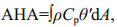 (10)
(10)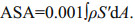 (11)
(11)The available dissolved oxygen anomalies (AOA) is calculated by imitating the formula of ASA. The unit of dissolved oxygen anomaly field O' is mg/L, so each layer of AOA is defined as:
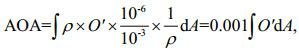 (12)
(12)where ρ is the density (kg/m3), Cp is the specific heat capacity (4 000 J/(kg∙K)), θ', S' and O' are the temperature, salinity, and dissolved oxygen anomaly fields, and A is the trapping area of the eddy. In this study, "trapping area" instead of core area above the trapping depth is used to estimate the heat, salinity, and oxygen transport. The result estimated by core area will be less than the actual value, because the water carried by eddy also includes the part whose swirl velocity exceeds the propagation speed (Ni, 2014).
Available heat anomalies in each layer of the mesoscale eddy during the three phases are shown in the Fig. 23. The highest heat transport anomaly value was located at 400–600 m depth. As the eddy developed, the AHA at each layer gradually increased, and the highest values is larger than 1×10¹⁷ J/m in the termination phase. Integrated from the surface to the trapping depth in each phase, the total AHA of the mesoscale eddy are 4.391×10¹⁷ J, 1.262×10¹⁸ J, 1.619×10¹⁸ J. Therefore, the heat transport caused by the eddy in each phase are 2.54×10¹¹ W, 7.30×10¹¹ W, 9.37×10¹¹ W, slightly larger than Ni's results. The heat transport was highest during the termination phase, and smallest during the initiation phase. The total heat transported by the eddy during the lifecycle was estimated to be about 5.89×10¹⁸ J.

|
| Fig.23 Available heat anomaly during three phases, the horizontal lines indicate the trapping depth |
Available salt anomalies in each layer of the mesoscale eddy during the three phases are shown in Fig. 24. At 500–600 m depth, ASA has a maximal value, and the value gradually increases with the development of eddy. In termination phase, it is larger than 1.2×10⁹ kg/m. Integrated from the surface to the trapping depth in each phase, the total ASA of the mesoscale eddy were -5.136×10⁹ kg, 8.081×10⁸ kg, 5.317×10⁹ kg. Therefore, the salt transport caused by the eddy during each phase was -2.97×10³ kg/s, 0.47×10³ kg/s, 3.08×10³ kg/s. The total salt transported by the eddy during the lifecycle was estimated to be about -1.36×10¹⁰ kg, indicating that the role of eddy is to reduce salinity in this region. Salt transport was highest during the termination phase, followed by the maturity phase, and lowest during the initiation phase. The magnitude of results are in consistent with Ni (2014) and Chaigneau et al. (2011), and our study presented the salt transport in a smaller time scale with negative value in the initiation phase and positive value in other two phases, while other research only provided a result of statistical data for a long time.

|
| Fig.24 Available salt anomaly during three phases, the horizontal lines indicate the trapping depth |
Available dissolved oxygen anomalies in three phases are shown in the Fig. 25. AOA gradually decreases with depth increasing, and the maximum value 2.8×10⁷ kg/m is at 100–200 m depth in the termination phase. Integrated from the surface to the trapping depth in each phase, the total AOA of the mesoscale eddy is 3.728×10⁸ kg, 4.007×10⁸ kg, 4.674×10⁸ kg. Moreover, the dissolved oxygen transport in each phase is 2.16×10² kg/s, 2.32×10² kg/s, 2.70×10² kg/s. The total dissolved oxygen transported by the eddy during the lifecycle was estimated to be about 2.76×10⁹ kg. Dissolved oxygen transport of the eddy was highest during the termination phase, followed by the maturity phase, and lowest during the initiation phase. The calculation result may make some contribution to the eddy's influence on the nutrient flux and biomass distribution.

|
| Fig.25 Available dissolved oxygen anomaly during three phases, the horizontal lines indicate the trapping depth |
The kinetic energy of an eddy is an important physical parameter for quantitatively describing its existence (Yang et al., 2019). It is considered to be closely related to the eddy's activity and plays an important role in its motion. The eddy kinetic energy can be calculated as: EKE=1/2(u2+v2), where u and v are the zonal and meridional velocity components, respectively. The eddy kinetic energy distribution during the seven periods are shown in the Fig. 26. The kinetic energy in the central region of the eddy was the lowest. The average eddy kinetic energy is 232 cm2/s2 during its lifetime, which is close to statistic result of 300 cm2/s2 in the northwestern subtropical Pacific Ocean obtained by Yang et al. (2013). In the area surrounding the center, the kinetic energy was high, reaching a maximum value of 1 630 cm2/s2. During the termination phase, the regions with high eddy kinetic energy are mainly distributed in the northeast.

|
| Fig.26 Kinetic energy changes during the eddy's lifetime |
The anticyclonic eddy had an average radius of 91.6 km, which was slightly smaller than the statistical result of 121 km in the northwestern subtropical Pacific Ocean by Yang et al. (2013). The interaction between the eddy and Izu Ridge led to a greatly enhance and a rapid drop of radius. McWilliams and Flierl (1979) concluded that when eddies reach the ridge in a status called "deep compensation"; there is no motion in phase with the upper layer in the lower layer. The eddy would lead to the reorganization of eddies' vertical structure, allowing the upper layer to cross the ridge without further influences (Beismann et al., 1999). From the sections 3.3 to 3.5, the eddy remained a relatively stable vertical structure during the lifecycle and the core is distinguishable as a coherent feature. When the eddy reached the Izu Ridge, it had not switched to the "deep compensation" status. From the anomalous geostrophic flow velocity, we can see the velocity field in the termination phase had a decline. However, from the slice and profile of temperature, salinity, dissolved oxygen, the decline was not obvious. Therefore, the loss of deep eddy structure was not obvious for this eddy. The eddy propagation speed and direction are strongly influenced by the Izu ridge, and finally being blocked and dissipated over the ridge.
The mesoscale eddy had a temperature and salinity anomaly core at 400–600 m. Its average temperature and salinity anomaly value Δθ, ΔS was +2.5℃, 0.15, respectively. It shows a stronger structure compared with the eddies in the Kuroshio Extension region studied by Sun et al. (2017), which shows that maximum warming in AE reaches 1.78℃ at 410 m of the eddy core, with maximum salinity change of 0.12 at 260 m. The mesoscale eddy in this study remained at the potential density layer of 25.5–26 kg/m3 during the lifetime, suggesting that the water trapped in the eddy core maintain a relatively stable state during the westward process of eddy. According to the character revealed by the composite structure (Figs. 6, 7, 10 & 11), we can conclude that the trapped water in core area had the temperature of 11–16℃, the salinity of 34.3–34.6. Therefore, according to the nature of the trapped water, we speculate that the trapped water might be originated from the L-CMW or the water mass with similar properties.
Oceanic mesoscale eddies contribute important horizontal heat and salt transports on a global scale (Dong et al., 2014). Dong et al. (2017) shows the distribution of eddy heat transport in the Northwestern Pacific Ocean from their method based on CH17 data. Zhang et al. (2014) used a new method combining the existing eddy trajectories, is applied to estimate heat and salt transports by eddy movements. For the first time, we present detailed temporal and spatial heat, salt, and dissolved oxygen transports by a single eddy with 17 Argo floats in the northwestern Pacific Ocean. In addition, many literatures composite the threedimensional structures with a series of different eddies in a region, which reflect the statistical characteristics. In this paper, we use the single eddy with in-situ observation data to do the work, and reflect its detailed three-dimensional structure during eddy's lifetime. To some extent, our results can supplement their findings, and show further detailed temporal variations of heat and salt transport during the eddy's lifecycle. In summary, the role of eddies in terms of heat and other anomalies, and the dynamic mechanism of the eddy need a deepened discussion. In the future, with more measured and in-situ data, we can make more analysis and some conclusions may be extended to the whole Northwest Pacific Ocean.
5 CONCLUSIONBy reconstructing the three-dimensional structure of an anticyclonic mesoscale eddy and analyzing its observed spatiotemporal variations in temperature, salinity, and oxygen field structure, the anomalous geostrophic flow velocity, heat, salt, and dissolved oxygen transport anomalies, and eddy kinetic energy are calculated and the features of the eddy and its interaction with the surroundings are better understood.
(1) The anticyclonic mesoscale eddy had a lifetime of 269 days and an average radius of 91.6 km. The eddy radius experienced a great enhance in the maturity phase, and had a rapid drop after entering the termination phase. The radius maximum reached 170 km in the maturity phase. The depth of its influence reached 1 000 m.
(2) The mesoscale eddy had a temperature and salinity anomaly core at 400–600 m. Its average temperature and salinity anomaly value Δθ, ΔS was +2.5℃, 0.15, respectively. From 800 to 900 m, a distinct low-salinity area was located at the center. The highest dissolved oxygen concentration anomaly was located at 200–300 m.
(3) Geostrophic flow velocity anomaly V was largest on the surface layer. V reached 0.3 m/s in the maturity phase. The maximum values of AHA, ASA, and AOA all occurred during the termination phase, which were about 1×10¹⁷ J/m, 1.2×10⁹ kg/m, 2.8×10⁷ kg/m, respectively. The total heat, salt and dissolved oxygen transported by the eddy during the lifecycle was estimated to be about 5.89×10¹⁸ J, -1.36×10¹⁰ kg, 2.76×10⁹ kg.
6 DATA AVAILABILITY STATEMENTThe datasets generated and analyzed during the current study are available from the corresponding author on reasonable request.
7 ACKNOWLEDGMENTWe thank reviewers for helpful suggestions. The program of eddy identification and tracking is from Dr. NI, and the program of calculating theoretical phase speed of Rossby waves is from Dr. WANG. The altimeter products used in this study are distributed by CMEMS (http://marine.copernicus.eu/).
Barth A, Beckers J M, Troupin C, Alvera-Azcárate A, Vandenbulcke L. 2014. Divand-1.0: n-dimensional variational data analysis for ocean observations. Geoscientific Model Development, 7(1): 225-241.
DOI:10.5194/gmd-7-225-2014 |
Beismann J O, Käse R H, Lutjeharms J R E. 1999. On the influence of submarine ridges on translation and stability of Agulhas rings. Journal of Geophysical Research: Oceans, 104(C4): 7 897-7 906.
DOI:10.1029/1998JC900127 |
Busireddy N K R, Osuri K K, Sivareddy S, Venkatesan R. 2018. An observational analysis of the evolution of a mesoscale anti-cyclonic eddy over the Northern Bay of Bengal during May-July 2014. Ocean Dynamics, 68(11): 1 431-1 441.
DOI:10.1007/s10236-018-1202-4 |
Chaigneau A, Gizolme A, Grados C. 2008. Mesoscale eddies off Peru in altimeter records: Identification algorithms and eddy spatio-temporal patterns. Progress in Oceanography, 79(2-4): 106-119.
DOI:10.1016/j.pocean.2008.10.013 |
Chaigneau A, Eldin G, Dewitte B. 2009. Eddy activity in the four major upwelling systems from satellite altimetry (1992-2007). Progress in Oceanography, 83(1-4): 117-123.
DOI:10.1016/j.pocean.2009.07.012 |
Chaigneau A, Le Texier M, Eldin G, Grados C, Pizarro O. 2011. Vertical structure of mesoscale eddies in the eastern South Pacific Ocean: A composite analysis from altimetry and Argo profiling floats. Journal of Geophysical Research Oceans, 116(C11): C11025.
DOI:10.1029/2011JC007134 |
Chelton D B, De Szoeke R A, Schlax M G, El Naggar K, Siwertz N. 1998. Geographical variability of the first baroclinic Rossby radius of deformation. Journal of Physical Oceanography, 28(3): 433-460.
DOI:10.1175/1520-0485(1998)028<0433:GVOTFB>2.0.CO;2 |
Chelton D B, Schlax M G, Samelson R M. 2011. Global observations of nonlinear mesoscale Eddies. Progress in Oceanography, 91(2): 167-216.
DOI:10.1016/j.pocean.2011.01.002 |
Chen G X, Hou Y J, Chu X Q. 2011. Mesoscale eddies in the South China Sea: mean properties, spatiotemporal variability, and impact on thermohaline structure. Journal of Geophysical Research: Oceans, 116(C6): C06018.
|
Dong C M, Lin X Y, Liu Y, Nencioli F, Chao Y, Guan Y P, Chen D K, Dickey T, Mcwilliams J C. 2012. Three-dimensional oceanic eddy analysis in the Southern California Bight from a numerical product. Journal of Geophysical Research: Oceans, 117(C7): C00H14.
DOI:10.1029/2011JC007354 |
Dong C M, Mcwilliams J C, Liu Y, Chen D K. 2014. Global heat and salt transports by eddy movement. Nature Communications, 5: 3 294.
DOI:10.1038/ncomms4294 |
Dong D, Brandt P, Chang P, Schütte F, Yang X F, Yan J H, Zeng J S. 2017. Mesoscale eddies in the northwestern Pacific Ocean: three-dimensional eddy structures and heat/salt transports. Journal of Geophysical Research: Oceans, 122(12): 9 795-9 813.
DOI:10.1002/2017JC013303 |
Furey H, Bower A, Perez-Brunius P, Hamilton P, Leben R. 2018. Deep eddies in the Gulf of Mexico observed with floats. Journal of Physical Oceanography, 48(11): 2 703-2 719.
DOI:10.1175/JPO-D-17-0245.1 |
Garreau P, Dumas F, Louazel S, Stegner A, Le Vu B. 2018. High-resolution observations and tracking of a dual-core anticyclonic eddy in the Algerian Basin. Journal of Geophysical Research: Oceans, 123(12): 9 320-9 339.
DOI:10.1029/2017JC013667 |
Huang E H, Pan D L, Li S J, He X Q. 2016. Comparing methods for identifying the outliers in the in-water profile spectral data. Journal of Marine Science, 24(1): 92-96.
(in Chinese with English abstract) |
Kamenkovich V M, Leonov Y P, Nechaev D A, Byrne D A, Gordon A L. 1996. On the Influence of bottom topography on the Agulhas eddy. Journal of Physical Oceanography, 26(6): 892-912.
DOI:10.1175/1520-0485(1996)026<0892:OTIOBT>2.0.CO;2 |
Keppler L, Cravatte S, Chaigneau A, Pegliasco C, Gourdeau L, Singh A. 2018. Observed characteristics and vertical structure of mesoscale eddies in the Southwest Tropical Pacific. Journal of Geophysical Research: Oceans, 123(4): 2 731-2 756.
DOI:10.1002/2017JC013712 |
Kusakabe M, Andreev A, Lobanov V, Zhabin I, Kumamoto Y, Murata A. 2002. Effects of the anticyclonic eddies on water masses, chemical parameters and chlorophyll distributions in the Oyashio current region. Journal of Oceanography, 58(5): 691-701.
DOI:10.1023/A:1022846407495 |
Lin X Y, Dong C M, Chen D K, Liu Y, Yang J S, Zou B, Guan Y P. 2015. Three-dimensional properties of mesoscale eddies in the South China Sea based on eddy-resolving model output. Deep Sea Research Part I: Oceanographic Research Papers, 99: 46-64.
DOI:10.1016/j.dsr.2015.01.007 |
Lin X Y, Guan Y P, Liu Y. 2013. Three-dimensional structure and evolution process of Dongsha cold eddy during autumn 2000. Journal of Tropical Oceanography, 32(2): 55-65.
(in Chinese with English abstract) |
Li J X, Wang G H, Xue H J, Wang H Z. 2019. A simple predictive model for the eddy propagation trajectory in the northern South China Sea. Ocean Science, 15(2): 401-412.
DOI:10.5194/os-15-401-2019 |
Ma X H, Jing Z, Chang P, Liu X, Montuoro R, Small R J, Bryan F O, Greatbatch R J, Brandt P, Wu D X, Lin X P, Wu L X. 2016. Western boundary currents regulated by interaction between ocean eddies and the atmosphere. Nature, 535(7613): 533-537.
DOI:10.1038/nature18640 |
McWilliams J C. 1985. Submesoscale, coherent vortices in the ocean. Reviews of Geophysics, 23(2): 165-182.
|
McWilliams J C. 2016. Submesoscale currents in the Ocean. Proceedings of the Royal Society A: Mathematical, Physical and Engineering Sciences, 472(2189): 20160117.
DOI:10.1098/rspa.2016.0117 |
McWilliams J C, Flierl G R. 1979. On the Evolution of Isolated, Nonlinear Vortices. Journal of Physical Oceanography, 9(6): 1 155-1 182.
DOI:10.1175/1520-0485(1979)009<1155:OTEOIN>2.0.CO;2 |
Nan F, Xue H J, Xiu P, Chai F, Shi M C, Guo P F. 2011. Oceanic eddy formation and propagation southwest of Taiwan. Journal of Geophysical Research: Oceans, 116(C12): C12045.
DOI:10.1029/2011JC007386 |
Nencioli F, Dong C M, Dickey T, Washburn L, McWilliams J C. 2010. A vector geometry-based eddy detection algorithm and its application to a high-resolution numerical model product and high-frequency radar surface velocities in the Southern California Bight. Journal of Atmospheric and Oceanic Technology, 27(3): 564-579.
DOI:10.1175/2009JTECHO725.1 |
Ni Q B. 2014. Statistical Characteristics and Composite Three-Dimensional Structures of Mesoscale Eddies Near the Luzon Strait. Xiamen University, Xiamen. (in Chinese with English abstract)
|
Oka E, Kouketsu S, Toyama K, Uehara K, Kobayashi T, Hosoda S, Suga T. 2011. Formation and subduction of central mode water based on profiling float data, 2003-08. Journal of Physical Oceanography, 41(1): 113-129.
|
Qiu C H, Mao H B, Wang Y H, Yu J C, Su D Y, Lian S M. 2018. An irregularly shaped warm eddy observed by Chinese underwater gliders. Journal of Oceanography, 75(2): 139-148.
|
Shu Y Q, Chen J, Li S, Wang Q, Yu J C, Wang D X. 2019. Field-observation for an anticyclonic mesoscale eddy consisted of twelve gliders and sixty-two expendable probes in the northern South China Sea during summer 2017. Science China Earth Sciences, 62(2): 451-458.
DOI:10.1007/s11430-018-9239-0 |
Shu Y Q, Xiu P, Xue H J, Yao J L, Yu J C. 2016. Glider-observed anticyclonic eddy in northern South China Sea. Aquatic Ecosystem Health & Management, 19(3): 233-241.
|
Song B, Wang H Z, Chen C L, Zhang R, Bao S L. 2019. Observed subsurface eddies near the Vietnam coast of the South China Sea. Acta Oceanologica Sinica, 38(4): 39-46.
DOI:10.1007/s13131-019-1412-8 |
Souza JMAC, de Boyer MC, Le Traon PY. 2011. Comparison between three implementations of automatic identification algorithms for the quantification and characterization of mesoscale eddies in the South Atlantic Ocean. Ocean Science, 7: 317-334.
DOI:10.5194/os-7-317-2011 |
Steinberg J M, Pelland N A, Eriksen C C. 2019. Observed evolution of a California Undercurrent eddy. Journal of Physical Oceanography, 49(3): 649-674.
DOI:10.1175/JPO-D-18-0033.1 |
Sun W J, Dong C M, Wang R Y, Liu Y, Yu K. 2017. Vertical structure anomalies of oceanic eddies in the Kuroshio Extension region. Journal of Geophysical Research Oceans, 122(2): 1 476-1 496.
DOI:10.1002/2016JC012226 |
Swart N C, Ansorge I J, Lutjeharms J R E. 2008. Detailed characterization of a cold Antarctic eddy. Journal of Geophysical Research: Oceans, 113(C1): C01009.
|
Troupin C, Barth A, Sirjacobs D, Ouberdous M, Brankart J M, Brasseur P, Rixen M, Alvera-Azcárate A, Belounis M, Capet A, Lenartz F, Toussaint M E, Beckers J M. 2012. Generation of analysis and consistent error fields using the Data Interpolating Variational Analysis (DIVA). Ocean Modelling, 52-53: 90-101.
DOI:10.1016/j.ocemod.2012.05.002 |
Wang G H, Su J L, Chu P C. 2003. Mesoscale eddies in the South China Sea observed with altimeter data. Geophysical Research Letters, 30(21): 2 121.
DOI:10.1029/2003GL018532 |
Wang Z F, Sun L, Li Q Y, Cheng H. 2019. Two typical merging events of oceanic mesoscale anticyclonic eddies. Ocean Science, 15(6): 1 545-1 559.
DOI:10.5194/os-15-1545-2019 |
Xie S P. 2013. Advancing climate dynamics toward reliable regional climate projections. Journal of Ocean University of China, 12(2): 191-200.
DOI:10.1007/s11802-013-2277-7 |
Xu L X, Li P L, Xie S P, Liu Q Y, Liu C, Gao W D. 2016. Observing mesoscale eddy effects on mode-water subduction and transport in the North Pacific. Nature Communications, 7: 10505.
DOI:10.1038/ncomms10505 |
Yang G, Wang F, Li Y L, Lin P F. 2013. Mesoscale eddies in the northwestern subtropical Pacific Ocean: Statistical characteristics and three-dimensional structures. Journal of Geophysical Research: Oceans, 118(4): 1 906-1 925.
DOI:10.1002/jgrc.20164 |
Yang Z B, Wang G H, Chen C L. 2019. Horizontal velocity structure of mesoscale eddies in the South China sea. Deep Sea Research Part I: Oceanographic Research Papers, 149: 103055.
DOI:10.1016/j.dsr.2019.06.001 |
Zhang W Z, Xue H J, Chai F, Ni Q B. 2015. Dynamical processes within an anticyclonic eddy revealed from Argo floats. Geophysical Research Letters, 42(7): 2 342-2 350.
DOI:10.1002/2015GL063120 |
Zhang Z G, Wang W, Qiu B. 2014. Oceanic mass transport by mesoscale eddies. Science, 345(6194): 322-324.
DOI:10.1126/science.1252418 |
Zhang Z W, Zhao W, Qiu B, Tian T W. 2017. Anticyclonic Eddy Sheddings from Kuroshio loop and the accompanying cyclonic eddy in the northeastern South China Sea. Journal of Physical Oceanography, 47(6): 1 243-1 259.
DOI:10.1175/JPO-D-16-0185.1 |