 2020, Vol. 38
Institute of Oceanology, Chinese Academy of Sciences
Article Information
- HU Yuyi, SHAO Weizeng, SHI Jian, SUN Jian, JI Qiyan, CAI Lina
- Analysis of the typhoon wave distribution simulated in WAVEWATCH-Ⅲ model in the context of Kuroshio and wind-induced current
- Journal of Oceanology and Limnology, 38(6): 1692-1710
- http://dx.doi.org/10.1007/s00343-019-9133-6
Article History
- Received May. 16, 2019
- accepted in principle Aug. 14, 2019
- accepted for publication Oct. 19, 2019


2 College of Meteorology and Oceanography, National University of Defense Technology, Nanjing 210007, China;
3 Physical Oceanography Laboratory, Ocean University of China, Qingdao 266100, China
It is well known that the Kuroshio is an important current in the northwest Pacific Ocean. In particular, this current advects high-temperature and highsalinity seawater from low latitudes in the Pacific Ocean to high-latitude seas, which has a huge impact on the meteorology, and hydrology of the oceans in these sea regions. To date, many studies have focused on the characteristics of the Kuroshio, e.g., the interannual variability of its entry into the South China Sea (Caruso et al., 2006). However, the interaction between currents and waves has not been well studied, especially in extreme conditions. Therefore, in this casework, we investigated the relationship between the wave distribution in typhoons and surface currents, including the Kuroshio and wind-induced currents. The typhoon-induced currents occupy the main part in wind-induced currents.
A typhoon-induced wave is a major cause of marine disasters, especially in coastal regions. Numerical wave models, e.g., the Wave Model (WAM) (The WAMDI Group, 1988), Simulating Waves Nearshore (SWAN) (Akpınar et al., 2012) and WAVEWATCH-Ⅲ (WW3) (Kim and Lee, 2018), as well as satellite observations, e.g., altimeter (Li et al., 2018) and synthetic aperture radar (SAR) (Li, 2015), are commonly used in studies of typhoon waves. The WW3 model, which was developed by the National Centers for Environmental Prediction (NCEP) of the National Oceanic and Atmospheric Administration (NOAA), has a good performance record for its wave simulation mode, with explicit treatment of nonlinear terms (Jiang et al., 2017). Moreover, the latest WW3 model (version 5.16) provides 3 convenient packages for the solution of the non-linear term quadruplets in the wave propagation equation (The WAVEWATCH Ⅲ Development Group, 2016). Until now, the WW3 model has been widely used for wave climate analysis (Gallagher et al., 2016), and it has been proved that this model has the capacity to simulate the waves of the Pacific Ocean (Bi et al., 2015; Zheng et al., 2016; Shukla et al., 2018), China Sea (He and Xu 2016; Zheng et al., 2018) and other critical seas (Gallagher et al., 2014; Guo et al., 2018). In particular, the WW3 model is also suitable for the study of typhoon waves (Sheng et al., 2018; Shao et al., 2018a). Moreover, the WW3 model provides a swap of the wave-current interaction, demonstrating that it has the capability to include the effect of currents.
Currently, most studies perform analyses of simulated typhoon waves (Fan et al., 2012; Montoya et al., 2013; Shao et al., 2018b), and the direct derivation of wave parameters, from satellite-based typhoon data (Shao et al., 2017; Ji et al., 2018), in which, to a certain extent, mesoscale dynamic processes, e.g., currents and eddies, are neglected. As proposed in Moon (2005), tides were found to be the most influential factor in modulating the mean wave characteristics in the Yellow and East China seas. The study by Cui et al. (2012) included a sensitivity analysis on the effect of ocean currents on typhoonwave modeling in East China Sea, and their results revealed sea surface currents have an effect on typhoon wave simulation. However, there have been few studies concerning typhoon waves in the open sea, where the sea surface currents play an important role, e.g., the Kuroshio and wind-induced currents.
Interestingly, the track of Typhoon Talim in 2017 was almost consistent with the Kuroshio track in the northwest Pacific Ocean. The typhoon lasted for 14 d and the minimum pressure dropped to nearly 940 hPa with wind speeds up to 50 m/s. Therefore, as a valuable case study, in this work, our goal was to investigate the performance of typhoon-induced waves within the context of the Kuroshio and a strong wind-induced current. The typhoon wave field was simulated using the latest WW3 model (version 5.16), and the simulated significant wave height (SWH) was validated against measurements from altimeter Jason-2. We then analyzed the relationship between background current and simulated typhoon wave distribution for the case study.
The remainder of this manuscript is organized as follows: data collection is introduced in Section 2; a description of the WW3 model and model setup are briefly described in Section 3; results are presented in Section 4; and the conclusions are summarized in Section 5.
2 DATA COLLECTIONThe typhoon data are provided by the Regional Specialized Meteorological Centre (RSMC), Tokyo-Typhoon Center of the Japan Meteorological Agency (JMA), which offers tropical cyclone information from the northwest Pacific Ocean. This information shows that Typhoon Talim existed from September 8 to 22, 2017. The tracks and maximum wind speeds of the typhoon associated with the bathymetric topography of the typhoon area are exhibited in Fig. 1a. The track of Typhoon Talim was clearly consistent with the flow of the Kuroshio. We also used the NCEP Climate Forecast System Version 2 (CFSv2) open-access surface current data from the National Center of Atmosphere Research (NCAR). The surface current field was 0.5°×0.5° gridded from August 1, 2017 to October 1, 2018 at 6-h intervals. As an example, Fig. 1b shows the CFSv2 surface current field on September 16, 2017 at 06:00 UTC. Of note, the maximum wind speed (up to 50 m/s) occurred when Talim passed the region of maximum surface current speed. Therefore, we interpret that the cyclonic pattern (Fig. 1b) is a wind-induced current, which exerted a more significant effect than the Kuroshio in this region.

|
| Fig.1 Bathymetric topography of the simulation area (a) and the map of NCEP Climate Forecast System Version 2 (CFSv2) currents (b) on September 16, 2017 at 06:00 UTC The black line represents the track of Typhoon Talim, provided by Tokyo-Typhoon Center of Japan Meteorological Agency (JMA), and the color dots in Fig. 1a represent the maximum wind speed of the typhoon. |
The European Centre for Medium-Range Weather Forecasts (ECMWF) now continuously provides global gridded atmospheric reanalysis data with a fine resolution of up to 0.125°×0.125° at 6-h intervals, which can be freely accessed from public datasets. ECMWF reanalysis data are widely used for oceanographic studies (Moeini et al., 2010; He et al., 2018), e.g., ECMWF wave data were a valuable source for verifying the results of the WW3 model in our previous study (Fan et al., 2012). However, due to the lack of individual wind-sea and swell information in these datasets, ERA-Interim wave data are not applicable for wave distribution analysis. Therefore, we utilized the WW3 model to simulate the typhoon wave field in this study, including total SWH, windsea SWH, and swell SWH.
The simulated area with 0.1°×0.1° gridded bathymetric topography from GEBCO (Weatherall et al., 2015) ranged from latitude 6°N to 44°N and longitude 111°E to 144°E. The model ran from August 1, 2017 to October 1, 2018. The ECMWF wind data on a 0.125° grid were taken as the forcing wind field. We also collected the measurements from altimeter Jason-2, which is popularly employed to validate numerical model simulations (Liu et al., 2016). When we collect the altimeter Jason-2 data, covering the WW3-simulated grids, the time difference between altimeter Jason-2 and simulations from WW3 model is within 15-min since the output of the WW3 model is set at 30-min. There were more than 7 000 matching points crossing the simulated area during the simulation period. As an example, the WW3- simulated significant wave height, overlaid by the matching points from altimeter Jason-2 on September 5, 2017 at 00:31 UTC is shown in Fig. 2, in which the points from altimeter Jason-2 are represented by colored rectangles. The altimeter-measured data are clearly close to the simulation results from the WW3 model. Furthermore, a statistical comparison demonstrated that the WW3-simulated SWHs agreed well with measurements collected by altimeter Jason-2, resulting in an RMSE equal to 0.34 m with a 0.45 scatter index (SI), as shown in Fig. 3. The SI calculation equation is,

|
| Fig.2 Map of WAVEWATCH-Ⅲ (WW3) significant wave height (SWH) overlaid by the points of satellite altimeter Jason-2 on September 5, 2017 at 00:31 UTC, represented by colored rectangles |

|
| Fig.3 Comparison between the simulated results and measurements from altimeter Jason-2 |
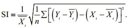 (1)
(1)We also found that WW3-simulate data generally underestimates the SWH, with a -0.30-m bias compared with altimeter measurements. This was probably caused by underestimated ECMWF winds, an interpretation that was consistent with the conclusion of Stopa and Cheng (2014). Regardless, we decided that the WW3-simulated wave fields could be reliable utilized in this study.
3 DESCRIPTION AND SETUP OF THE WW3 MODELIn this section, we provide a brief description of the WW3 model and the regular model setup. In particular, the selected options of the model are described, e.g., the input/dissipation terms and the nonlinear 4-wave component (quadruplet) wave-wave interactions, which play an important role in typhoon wave simulation.
3.1 Options of the WW3 modelThe WW3 model provides 7 input/dissipation terms, 4 nonlinear wave-wave interaction terms, and a nonlinear triad interaction. In our previous study (Shao et al., 2018b; Sheng et al., 2018), we found that these options were suitable for simulating the wave fields in Typhoon Talim, e.g., the input/dissipation terms, referred to as ST2 and STAB 2, and the Discrete Interaction Approximation (DIA) of nonlinear wavewave interactions.
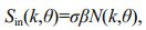
ST2 represents the input/dissipation term proposed by Tolman and Chalikov (1996). The atmospherewave interaction term Sin is proportional to the wave action density spectrum N, stated as,
 (2)
(2)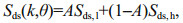 (3)
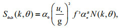
(3)where by k is the wave number, θ is the wave direction, β represents the non-dimensional wind-wave interaction parameter, σ is the high-frequency level, Sds, l is the low-frequency dissipation, Sds, h is the highfrequency dissipation, and A is the weighting coefficient determined by the wave frequency. Sds, l and Sds, h are defined as,
 (4)
(4) (5)
(5)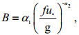 (6)
(6)where, h represents a scale factor determined by the high-frequency intrinsic energy of the wave field and ϕ is an empirical function which reflects the development stage of the wave field; u* is the wind velocity as the forcing field of the model; αn is a normalized Phillip's non-dimensional high-frequency energy level; α0=4.8, α1=1.7×10⁻⁴, and α2=2.0.
STAB 2 was devised by Tolman (2002) to stabilize the growth rate of deep-ocean waves in ST2. It primarily replaces the wind speed u* by an effective wind speed ue, which is stated as:
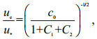 (7)
(7) (8)
(8) (9)
(9)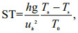 (10)
(10) (11)
(11)where, ST is a stability parameter, Ta is the air temperature, Ts is sea surface temperature, T0 is the reference temperature, and default parameters of c0=1.4, c1=-0.1, c2=0.1, c1=-0.1, f1=-150, and ST= -0.01 are implemented. It should be noted that the effective wind speed is measured at 10 m above the sea surface.
The DIA of the non-linear wave-wave interactions is a parameterization solution proposed initially in Hasselmann et al. (1985). The non-linear interactions are divided to quadruplets, with from wavenumber vectors k1 to k4. Under this condition, k1 is assumed to be equal to k2. Furthermore, resonance conditions require quadruplets to satisfy the following:
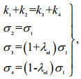 (12)
(12) (13)
(13) (14)
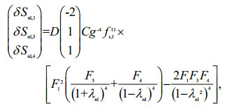
(14)where, λnl is a constant 0.25, and the relative frequencies σ1 to σ4 correspond to wavenumber vectors k1 to k4, respectively; δSnl represents the contribution to the interaction for each discrete spectrum F(fr, θ) combined with frequency and direction, and Eq. (The WAVEWATCH Ⅲ Development Group, 2016) corresponds to wavenumber k1, F1=F(fr, 1, θ), F(fr, 2, θ), …, δSnl, 1=δSnl(fr, 1, θ); and C=1.0×10⁷, c1=5.5, c2=5/6, and c3=1.25 are constants.
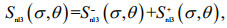
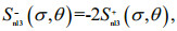
Nonlinear triad interactions were employed in this model, known as the GMD2 model, according to Liu et al. (2016), which is based on the Boussinesq-type deterministic equations proposed by Herterich and Hasselmann (1980). The equation for the nonlinear triad interactions is combined by adding and reducing the energy flux. The expression, suited for radian frequencies, is described as:
 (15)
(15) (16)
(16) (17)
(17) (18)
(18) (19)
(19)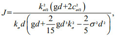 (20)
(20)where Snl3 represents the nonlinear triad interactions, Ur represents the local Ursell number, E is the spectral energy, σp is the self-interaction of the peak frequency, and αEB is set to a constant 0.05.
3.2 Setup of the WW3 modelThe 0.125°-gridded ECMWF winds, the 0.5°-gridded CFSv2 currents were taken as the forcing field, and the GEBCO bathymetric data consisted of a 30 arc-second gird. These data were bilinearly interpolated into gridded data with a 1° spatial resolution. Thus, the WW3-simulated waves with a 1° grid are taken as the open boundary over the global seas.
The regional simulated area ranged from latitude 6°N to 44°N and longitude 111°E to 144°E. The ECMWF winds and GEBCO data were interpolated to 0.5° grids, which had the same spatial resolution as the NCEP CFSv2 current field. The two-dimensional wave spectrum was resolved into 24 regular azimuthal directions, in which the wave frequency of the bins logarithmically ranged from 0.041 18 to 0.718 6 at an interval of Δf/f=0.1, and the time step of the spatial propagation was determined to be 300 s for both the latitudinal and longitudinal directions. The resolution of the model output was 0.1°-gridded.
4 RESULTFigure 4 shows the daily average results of SWH from September 13 to 16, 2017, during which time the track of Typhoon Talim almost overlaid the Kuroshio. This figure shows that the high SWH appeared in the same area. As time passed, the high SWH area moved with the typhoon. In addition, it was found that the maximum SWH reached 10 m in the East China Sea on September 14, which was consistent with the maximum current speed for the region (about 1.5 m/s) induced by strong winds, as shown in Fig. 5. Interestingly, the pattern of the simulated SWH was similar to that of current. Moreover, the SWH was larger to the east of Taiwan, China, than to the west, as can clearly be observed in Fig. 5c & d. Figure 6 shows the average surface relative vorticity from September 13 to 16, the pattern of which was inconsistent with the simulated wave field from the WW3 model. Interestingly, the tendency of surface relative vorticity area is inconsistent with that of the SWH. This phenomenon is clearly observed in the Fig. 6a.

|
| Fig.4 Average SWH on September 13 (a), September 14 (b), September 15 (c), and September 16 (d) |

|
| Fig.5 Average current speed provided by NCEP Climate Forecast System Version 2 (CFSv2) from 00:00 UTC September 13 to 00:00 UTC September 17, 2017 a. September 13; b. September 14; c. September 15; d. September 16. |

|
| Fig.6 Average current surface relative vorticity, calculating by NCEP Climate Forecast System Version 2 (CFSv2) data, from 00:00 UTC September 13 to 00:00 UTC September 17, 2017 a. September 13; b. September 14; c. September 15; d. September 16. |
Figure 7 shows the average wave length at peak from September 13 to 16, which revealed that the average wave length distribution was inconsistent with the simulated wave field from the WW3 model, particularly in Fig. 7c & d. The average wave peak speed from September 13 to 16 is shown in Fig. 8 and exhibited no obvious relationship with the simulated wave field from the WW3 model. The average wave steep rate from September 13 to 16 displayed a high correlation with the simulated wave field from the WW3 model, as shown in Fig. 9. Overall, we determined that there is a positive correlation between surface current speeds and typhoon waves.

|
| Fig.7 Average wave length at peak from 00:00 UTC September 13 to 00:00 UTC September 17, 2017 a. September 13; b. September 14; c. September 15; d. September 16. |

|
| Fig.8 Average wave peak speeds, calculating by the WW3 model data, from 00:00 UTC September 13 to 00:00 UTC September 17, 2017 a. September 13; b. September 14; c. September 15; d. September 16. |

|
| Fig.9 Average wave steep rate, calculating by the WW3 model data, from 00:00 UTC September 13 to 00:00 UTC September 17, 2017 a. September 13; b. September 14; c. September 15; d. September 16. |
To better illustrate the relationship between surface current speed, e.g., Kuroshio and the wind-induce current, and SWH, we chose 6 points for further analysis. The geographic locations of these points are shown in Fig. 10. The 2 points A and C are located to the east of Taiwan, China, where the Kuroshio exists. The 2 points B and D are located on either side of the track of Typhoon Talim in areas with maximum SWH. The last 2 points, E and F, are close to Japan, with F also located in the Kuroshio region. The black rectangle encloses the area used to generate the scatter plot shown in the Fig. 11, which depicts the relationship between surface current speed and SWH. As shown in Fig. 11a, the surface current speed and SWH have a correlation of 0.75. Thus, this indicates that the current speed is positively related to the typhoonassociated SWH. In the Fig. 11b, we can find that the surface current direction is not directly related with the typhoon-associated SWH. Moreover, it is no obvious relationship between surface current direction and wave direction in Fig. 11c & d.

|
| Fig.10 Average surface current speed provided by NCEP Climate Forecast System Version 2 (CFSv2), from September 13 to 17, 2017 The black line represents the track of typhoon Talim, and the 6 white dots (A to F) represent the points selected for analysis. The black rectangle encloses the areas used to generate the scatter plot in Fig. 11. |

|
| Fig.11 Comparison between surface current speed and SWH from the WW3 model (a); comparison between surface current direction and SWH from the WW3 model (b); comparison between surface current direction and mean wave direction from the WW3 model (c); comparison between surface current direction and wave direction at peak from the WW3 model (d) For the area enclosed within covering the black rectangle in Fig. 10. |
The relationship between surface current speed and SWH can be seen in Fig. 12. At points A and C, located in the Kuroshio, it was found that the SWH exhibited a similar trend to that of the change in surface current speed during the duration of typhoon from September 11 to 20. This relationship is particularly evident in Fig. 12b & d, when the SWH reached 11 m and the surface current speed exceeded 1 m/s. Although, the current speed were approximately 0.2 and 0.4 m/s at the beginning of Typhoon Talim for points A and C, respectively, the tendency of surface current is similar to that of the SWH. In addition, Fig. 12c & e show the surface current speed to be around 0.5 m/s before September 11 without any strong wind-induced current, indicating that the surface current is to some extent related to the SWH. However, as shown in Fig. 12a & f, the relationship between surface current and SWH is weak, and not significant, at surface current speeds smaller than 0.2 m/s. Other points A, C, E, and F show less significant relation between SWH and current, which is nearby the land. Collectively, these results indicate that the effect of surface current on wave simulation should be considered when the surface current speed is greater than 0.5 m/s. In particular, the wave-current interaction term is important for wave simulation in typhoons.

|
| Fig.12 Relationship between significant wave height and surface current speed with time from 00:00 UTC September 1 to 00:00 UTC September 21, 2017 a–f represent the data from the points A–F in Fig. 10. |
The wind-sea and swell data from the WW3 model can be simulated separately and widely used for studying the wind-sea and swell distributions across the global seas (Bi et al., 2015; Gallagher et al., 2016). To further study the interaction between surface current and wave, we divided the wave system into individual wind-sea and swell components. As an example, Fig. 13 shows the average wind-sea SWH from the WW3 model. As seen in the figure, from September 14 the maximum wind-sea SWH reached nearly 8 m. Figure 14 shows the average swell SWH, for which the maximum swell SWH was less than 6 m. It was discovered that the wind-sea components dominate around the typhoon eye, while swells dominate outside the eye. It was also discovered that the distribution of surface current speed was consistent with that of wind-sea SWH in the East China Sea, a consistency that was particularly pronounced in Fig. 13b & c.

|
| Fig.13 Average wind-sea significant wave height from September 13 to September 16, 2017 a. September 13; b. September 14; c. September 15; d. September 16. |

|
| Fig.14 Averaged swell significant wave height from September 13 to September 16, 2017 a. September 13; b. September 14; c. September 15; d. September 16. |
The same points A–F were used to analyze windsea and swell against the backdrop of surface current over the entire duration of the typhoon, as shown in Figs. 15 & 16, respectively. It can be clearly observed that the trend of the surface current was consistent with the wind-sea trend from September 13 to 16 in Fig. 15b (point B) and d (point D). The relationship between swell and surface current speed, however, is messy, as shown in Fig. 16b & d. At points C and E, swell dominates from 13 to 16 September, and the relationship between surface current and swell is weak. Again, there is no close correlation between the current and SWH at low current speeds (points A and F). This analysis demonstrates that the interaction of the surface current with the distribution of typhoon waves most likely derives from the wind-sea component of the wave system. Although the pattern of wind-induced current is consistent with that of wind-sea, the dynamics between surface currents and waves needs to be further studied because the processes in the interaction between wind-sea and current is complicated, e.g., exchange of energy, heat and spray.

|
| Fig.15 Relationship between wind-sea significant wave height and surface current speed with time from September 1 to 21, 2017 a–f represent the data from points A–F in Fig. 10. |

|
| Fig.16 Relationship between swell significant wave height and surface current speed with time from September 1 to 21, 2017 a–f represent the data from points A–F in Fig. 10. |
Wave-current interactions are often ignored in wave simulations of typhoons. However, the Kuroshio plays an important role in the open sea of the western Pacific. In addition, strong winds in typhoons can induce currents. It was found that the track of Typhoon Talim was almost consistent with the Kuroshio from September 13 to 16, 2017. In this case study, we investigated the applicability of the latest version of the WW3 model (version 5.16) and analyzed typhooninduced waves while considering the surface current terms, including the Kuroshio and wind-induced current. It is noted that the wind-induced current (up to 1.5 m/s) was stronger than Kuroshio around typhoon eye. However, in regions far from the eye or with weak winds, the Kuroshio dominated.
In this study, SWHs were simulated using the WW3 model from August 1, 2017 to October 1 2018, including a term for the wave-current interaction. ECMWF winds on a 0.125°-grid and surface current data from CFSv2 on a 0.5°-grid comprised the forcing field. We used measurements from altimeter Jason-2 to validate the simulated SWH, which revealed a 0.34-m RMSE of SWH with a 0.45-m SI. It was observed that SWH is positively correlated with wind-induced current speed, while there is no relationship between SWH and several wave parameters, e.g., surface relative vorticity, wavelength at peak and wave peak speed. The trend of the Kuroshio was also consistent with the change of SWH and wave steep rate at current speeds greater than 0.5 m/s. However, it is difficult to draw any definitive conclusions for surface current speeds lower than 0.2 m/s.
The distributions of wind-sea and swell were analyzed in the context of surface current. The windsea pattern was consistent with the typhoon-induced surface current, while there was a weak relationship between surface current and swell. In summary, we conclude that there is a positive correlation between surface current speed, including that of the Kuroshio and strong wind-induced current, and typhoon waves. In the near future, we plan to simulate waves with the WW3 model in the context of surface currents, utilizing the various tracks of typhoons that have occurred over the past 20 years around the China Sea. The climate associated with typhoon-induced waves will be analyzed; in particular, the dynamics between surface currents and the development wind-sea components will be investigated in greater detail.
6 DATA AVAILABILITY STATEMENTAll data generated and/or analyzed during this study are available from the corresponding author on reasonable request.
7 ACKNOWLEDGMENTWe appreciate the National Centers for Environmental Prediction (NCEP) of the National Oceanic and Atmospheric Administration (NOAA) for providing the source code for the WAVEWATCH-Ⅲ (WW3) model. The European Centre for MediumRange Weather Forecasts (ECMWF) wind data were accessed via http://www.ecmwf.int. The General Bathymetry Chart of the Oceans (GEBCO) data were downloaded via: ftp.edcftp.cr.usgs.gov. Current field data from the NCEP Climate Forecast System Version 2 (CFSv2) were collected via http://cfs.ncep.noaa.gov. The Operational Geophysical Data Record (OGDR) wave data from the altimeter Jason-2 mission were accessed via https://data.nodc.noaa.gov. Typhoon parameters were provided by the Japan Meteorological Agency (JMA) via http://www.jma.go.jp.
Akpınar A, Van Vledder G P, Kömürcü M İ, Özger M. 2012. Evaluation of the numerical wave model (SWAN) for wave simulation in the Black Sea. Continental Shelf Research, 50-51: 80-99.
DOI:10.1016/j.csr.2012.09.012 |
Bi F, Song J B, Wu K J, Xu Y. 2015. Evaluation of the simulation capability of the Wavewatch Ⅲ model for Pacific Ocean wave. Acta Oceanologica Sinica, 34(9): 43-57.
DOI:10.1007/s13131-015-0737-1 |
Caruso M J, Gawarkiewicz G G, Beardsley R C. 2006. Interannual variability of the Kuroshio intrusion in the South China Sea. Journal of Oceanography, 62(4): 559-575.
DOI:10.1007/s10872-006-0076-0 |
Cui H, He H L, Liu X H, Li Y. 2012. Effect of oceanic current on typhoon-wave modeling in the East China Sea. Chinese Physics B, 21(10): 109201.
DOI:10.1088/1674-1056/21/10/109201 |
Fan Y, Lin S J, Held I M, Yu Z T, Tolman H L. 2012. Global ocean surface wave simulation using a coupled atmosphere-wave model. Journal of Climate, 25(18): 6 233-6 252.
DOI:10.1175/JCLI-D-11-00621.1 |
Gallagher S, Gleeson E, Tiron R, Mcgrath R, Dias F. 2016. Wave climate projections for Ireland for the end of the 21st century including analysis of EC—Earth winds over the North Atlantic Ocean. International Journal of Climatology, 36(14): 4 592-4 607.
DOI:10.1002/joc.4656 |
Gallagher S, Tiron R, Dias F. 2014. A long-term nearshore wave hindcast for Ireland: Atlantic and Irish Sea coasts (1979-2012). Ocean Dynamics, 64(8): 1 163-1 180.
DOI:10.1007/s10236-014-0728-3 |
Guo L L, Perrie W, Long Z C, Toulany B, Sheng J Y. 2018. The impacts of climate change on the autumn North Atlantic wave climate. Atmosphere-Ocean, 53(5): 491-509.
|
Hasselmann S, Hasselmann K, Allender J H, Barnett T P. 1985. Computations and parameterizations of the nonlinear energy transfer in a gravity-wave spectrum. Part Ⅱ: Parameterizations of the nonlinear energy transfer for application in wave models. Journal of Physical Oceanography, 15(11): 1 378-1 391.
DOI:10.1175/1520-0485(1985)015<1378:CAPOTN>2.0.CO;2 |
He H L, Song J B, Bai Y, Xu Y, Wang J J, Fan B. 2018. Climate and extrema of ocean waves in the East China Sea. Science China Earth Sciences, 61(7): 980-994.
DOI:10.1007/s11430-017-9156-7 |
He H L, Xu Y. 2016. Wind-wave hindcast in the Yellow Sea and the Bohai Sea from the year 1988 to 2002. Acta Oceanologica Sinica, 35(3): 46-53.
DOI:10.1007/s13131-015-0786-5 |
Herterich K, Hasselmann K. 1980. A similarity relation for the nonlinear energy transfer in a finite-depth gravity-wave spectrum. Journal of Fluid Mechanics, 97(1): 215-224.
DOI:10.1017/S0022112080002522 |
Ji Q Y, Shao W Z, Sheng Y X, Yuan X Z, Sun J, Zhou W, Zuo J C. 2018. A promising method of typhoon wave retrieval from Gaofen-3 synthetic aperture radar image in VV-polarization. Sensors, 18(7): 2 064.
DOI:10.3390/s18072064 |
Jiang C B, Zhao B B, Deng B, Wu Z Y. 2017. Numerical simulation of typhoon storm surge in the Beibu Gulf and hazardous analysis at key areas. Marine Forecasts, 34(3): 32-40.
(in Chinese with English abstract) |
Kim T R, Lee J H. 2018. Comparison of high wave hindcasts during Typhoon Bolaven (1215) using SWAN and WAVEWATCH Ⅲ model. Journal of Coastal Research, 85(sp1): 1 096-1 100.
|
Li S Q, Guan S D, Hou Y J, Liu Y H, Bi F. 2018. Evaluation and adjustment of altimeter measurement and numerical hindcast in wave height trend estimation in China's coastal seas. International Journal of Applied Earth Observation and Geoinformation, 67: 161-172.
DOI:10.1016/j.jag.2018.01.007 |
Li X F. 2015. The first Sentinel-1 SAR image of a typhoon. Acta Oceanologica Sinica, 34(1): 1-2.
DOI:10.1007/s13131-015-0589-8 |
Liu Q X, Babanin A V, Zieger S, Young I R, Guan C L. 2016. Wind and wave climate in the Arctic ocean as observed by altimeters. Journal of Climate, 29(22): 7 957-7 975.
DOI:10.1175/JCLI-D-16-0219.1 |
Moeini M H, Etemad-Shahidi A, Chegini V. 2010. Wave modeling and extreme value analysis off the northern coast of the Persian Gulf. Applied Ocean Research, 32(2): 209-218.
DOI:10.1016/j.apor.2009.10.005 |
Montoya R D, Arias A O, Royero J C O, Ocampo-Torres F J. 2013. A wave parameters and directional spectrum analysis for extreme winds. Ocean Engineering, 67: 100-118.
DOI:10.1016/j.oceaneng.2013.04.016 |
Moon I J. 2005. Impact of a coupled ocean wave-tide-circulation system on coastal modeling. Ocean Modelling, 8(3): 203-236.
DOI:10.1016/j.ocemod.2004.02.001 |
Shao W Z, Hu Y Y, Yang J S, Nunziata F, Sun J, Li H, Zuo J C. 2018a. An empirical algorithm to retrieve significant wave height from Sentinel-1 synthetic aperture radar imagery collected under cyclonic conditions. Remote Sensing, 10(7): 1 367.
|
Shao W Z, Li X F, Hwang P A, Zhang B, Yang X F. 2017. Bridging the gap between cyclone wind and wave by C-band SAR measurements. Journal of Geophysical Research: Oceans, 122(8): 6 714-6 724.
DOI:10.1002/2017JC012908 |
Shao W Z, Sheng Y X, Li H, Shi J, Ji Q Y, Tai W, Zuo J C. 2018b. Analysis of wave distribution simulated by WAVEWATCH-Ⅲ model in typhoons passing Beibu Gulf, China. Atmosphere, 8(7): 265.
|
Sheng Y X, Shao W Z, Li S Q, Zhang Y M, Yang H W, Zuo J C. 2018. Evaluation of typhoon waves simulated by WaveWatch-Ⅲ model in shallow waters around Zhoushan islands. Journal of Ocean University of China, 18(2): 365-375.
|
Shukla R P, Kinter J L, Shin C S. 2018. Sub-seasonal prediction of significant wave heights over the Western Pacific and Indian Oceans, part Ⅱ: The impact of ENSO and MJO. Ocean Modelling, 123: 1-15.
DOI:10.1016/j.ocemod.2018.01.002 |
Stopa J E, Cheung K F. 2014. Intercomparison of wind and wave data from the ECMWF reanalysis interim and the NCEP climate forecast system reanalysis. Ocean Modelling, 75: 65-83.
DOI:10.1016/j.ocemod.2013.12.006 |
The WAMDI Group. 1988. The WAM Model—a third generation ocean wave prediction model. Journal of Physical Oceanography, 18(12): 1 775-1 810.
DOI:10.1175/1520-0485(1988)018<1775:TWMTGO>2.0.CO;2 |
The WAVEWATCH Ⅲ Development Group (WW3DG). 2016. User Manual and System Documentation of WAVEWATCH Ⅲ Version 5. 16. 329p; Technical Note, MMAB Contribution; NOAA/NWS/NCEP/MMAB: College Park, MD, USA; Volume 276, 326p.
|
Tolman H L. 2002. Validation of WAVEWATCH Ⅲ Version 1.15 for a Global Domain. NCEP Technical Note 213. National Oceanic and Atmospheric Administration, Camp Springs, US. 213p.
|
Tolman H L, Chalikov D V. 1996. Source terms in a third-generation wind wave model. Journal of Physical Oceanography, 26(11): 2 497-2 518.
DOI:10.1175/1520-0485(1996)026<2497:STIATG>2.0.CO;2 |
Weatherall P, Marks K M, Jakobsson M, Schmitt T, Tani S, Arndt J E, Rovere M, Chayes D, Ferrini V, Wigley R. 2015. A new digital bathymetric model of the world's oceans. Earth and Space Science, 2(8): 331-345.
|
Zheng K W, Sun J, Guan C L, Shao W Z. 2016. Analysis of the global swell and wind sea energy distribution using WAVEWATCH Ⅲ. Advances in Meteorology, 2016: 8419580.
|
Zheng K W, Osinowo A A, Sun J, Hu W. 2018. Long-term characterization of sea conditions in the East China Sea using significant wave height and wind speed. Journal of Ocean University of China, 17(4): 733-743.
DOI:10.1007/s11802-018-3484-z |