 2020, Vol. 38
Institute of Oceanology, Chinese Academy of Sciences
Article Information
- WANG Huizan, LIU Ding, ZHANG Weimin, LI Jiaxun, WANG Bo
- Characterizing the capability of mesoscale eddies to carry drifters in the northwest Pacific
- Journal of Oceanology and Limnology, 38(6): 1711-1728
- http://dx.doi.org/10.1007/s00343-019-9149-y
Article History
- Received May. 31, 2019
- accepted in principle Aug. 1, 2019
- accepted for publication Dec. 2, 2020


2 Naval Research Academy, Tianjin 300061, China
Mesoscale eddies are nearly ubiquitous throughout oceans, usually range from 10 to 100 km in diameter and persist from days to months. At present, knowledge of mesoscale eddy is gradually deepening because a variety of ocean observation methods are currently available. An eddy study often begins with eddy identification, for which various data are used for the detection, such as sea surface height (SSH), sea surface temperature (SST), chlorophyll concentration, and sea surface velocity. Of these data, sea surface height (SSH) data are the most widely applied (Wang et al., 2003, 2019a, 2019b; Jia and Liu, 2004; Chelton et al., 2011; Duo et al., 2019; Li et al., 2019). In the past 20 years, extensive studies focused on eddy identification, statistical characteristics, and the structure and transport of mass, heat, and salt, but the ability of mesoscale eddies to carry real particles has not been addressed well. Zhang et al. (2015) investigated the dynamical processes within an anticyclonic eddy with the combination of Sea Level Anomaly (SLA) data and Argo data, where Argo floats revealed the motion of particles in anticyclonic eddies, by which this study was inspired.
Many studies about mesoscale eddies in the northwest Pacific or its subregions revealed their features and structures (Yang et al., 2013; Qiu et al., 2014; Zheng et al., 2014; Dong et al., 2017; Dai et al., 2019). For example, Yang et al. (2013) found that eddy occurrence frequency is prevailingly high in the Subtropical Countercurrent zonal band between 19°N and 26°N. Zheng et al. (2014) found that the offshore northwest Pacific, northern Kuroshio Extension, Subtropical Counter Current are high frequency of eddy occurrence, and the distribution of eddy polarity shows a difference in the south (north) of the 35°N with more cyclonic eddies (anticyclonic eddies). Dong et al. (2017) studied the three-dimensional structures and transports of mesoscale eddies in Northwestern Pacific Ocean encompassing the Kuroshio Extension (KE) by combining satellite data with Argo profiles. Dai et al. (2020) studied spatiotemporal variation of the three-dimensional structure and heat/salt transport of an anticyclonic mesoscale eddy based on 17 Argo floats in the northwest Pacific.
Satellite-tracked drifting buoys (hereafter referred to as "drifters") of the Global Drifter Program (GDP) have been collecting near-surface ocean current observations since 1979. Since these drifters have a drogue (sea anchor) centered at the depth of 15 m, their trajectories thus reflect the motion of nearsurface ocean currents (Niiler, 2001; Lumpkin and Pazos, 2007), and the total current measured by a drifter comprises the geostrophic current, the Ekman current, and a number of other ageostrophic currents (Rio, 2012; Zhang and Qiu, 2018).
Previous studies combining drifter and mesoscale eddy data focused on eddy identification based on drifter trajectories (Dong et al., 2011; Li et al., 2011) and the investigation of eddy's surface velocity (Zhang and Qiu, 2018; de Marez et al., 2019). For example, Li et al. (2011) detected eddies in the northern South China Sea from drifter trajectories (1979–2010) using a geometric method, statistically characterized the spatial and temporal patterns of mesoscale eddies, and then revealed the relationship between the patterns and the sea surface height anomaly (SSHA). Using the global surface velocity measurements by drifters, Zhang and Qiu (2018) showed that the submesoscale ageostrophic kinetic energy exhibits unexpected global-mean features through the life cycle of mesoscale eddies.
As a single drifter can be treated as a real particle due to its water-following feature, it is also possible to investigate the ability of mesoscale eddies to carry drifters by colocalizing the drifters and eddies. In this study, by combining the SLA data and the drifter data in the northwest Pacific (99°E–180°E, 0°–66°N) from 1993 to 2015, the method of colocalization and composite analysis were used to characterize the capability of mesoscale eddies (identified from the SLA data) to carry drifters. The interpretation of the carrying capability of eddies was also provided by introducing Rossby number.
The paper is organized as follows: Section 2 describes the data and methods employed in this study; Section 3 investigates the statistical characteristics of carrying process and discusses the mechanisms. The conclusions are presented in Section 4.
2 DATA AND METHOD 2.1 DataSLA data were employed for mesoscale eddy identification. The satellite altimetry data used in this study were obtained from the sea level anomaly delayed-time product recorded from January 1993 to December 2015 in the northwest Pacific (99°E–180°E, 0°–66°N). These SLA data have a spatial resolution of 0.25°×0.25° with an one-day interval. The data are distributed by the Archiving Validation and Interpretation of Satellite Data in Oceanography (AVISO) supported by the Centre National d'Études Spatiales (CNES) of France (http://www.aviso.altimetry.fr/en/data/products/sea-surface-height-products/global.html). As the data contain aliases over the shelf area (Yuan et al., 2006), the records of eddy over the shelf shallower than 200 m were removed.
The Global Drifter Program (GDP) satellitetracked quality-controlled 6-hourly interpolated data from ocean surface drifting buoys are provided by the National Oceanic and Atmospheric Administration (NOAA) (ftp://ftp.aoml.noaa.gov/pub/phod/buoydata/), and drifters in the northwest Pacific from 1993 to 2015 were selected. In this study, the primary drifter data contain the information of longitude, latitude, and time (6-hourly). The drifter data with position (drifter trajectories) were used to be colocalized with the eddies for studying the eddy carrying capability. The spurious low-frequency variability in drifter velocities was removed (Lumpkin et al., 2013) before the study and very few drifter data were interpolated in the case of record missing in the study. Drifter motion is mainly affected by sea surface velocity and wind speed. Drifting caused by wind is known as the downwind "slip" (drifter motion with respect to water motion at a depth of 15 m), which is only ~0.1% of the wind speed for winds up to 10 m/s (Niiler et al., 1995). Therefore, drifters can be regarded as particles that are carried along with the current and have little relationship with the wind speed impact.
The daily sea-surface geostrophic velocity anomaly data were employed in the composite of eddy velocity field. The daily surface geostrophic eastward and northward seawater velocity assuming sea level for geoid (geostrophic velocity anomaly u′ and v′) were provided by the Copernicus Marine Environment Monitoring Service (CMEMS) (http://marine.copernicus.eu/). The Global ocean gridded L4 Sea Surface Heights and Derived Variables Reprocessed Product are gridded on a grid of 0.25×0.25° with temporal resolution of one day. This product was processed by the SL-TAC multimission altimeter data processing system. It processes data from all altimeter missions: Jason-3, Sentinel-3A, HY-2A, Saral/AltiKa, Cryosat-2, Jason-2, Jason-1, T/P, ENVISAT, GFO, and ERS1/2. The geostrophic velocity anomaly is derived from SLA data computed with an optimal and centered computation time window (6 weeks before and after the date).
2.2 Eddy identification and tracking methodsThe method of eddy identification and tracking used in this paper were employed by Ni (2014), Wang et al. (2018), and Zhang et al. (2018). The SLA contour-based eddy identification method was modified from two similar methods applied by Chaigneau et al. (2009) and Chelton et al. (2011). In detail, the SLA contour lines (isolines), which stand for different values of the SLA, are plotted at an interval of 0.5 cm (Zhang et al., 2018). The geometric innermost closed contour is treated as the eddy center and the outermost closed contour as the eddy edge. Taking one SLA map of an area in the northwest Pacific as an example, eddy identified from it is based on the above-mentioned method as presented in Fig. 1. The method is superior to the Okubo-Weiss method in the aspect of accuracy and correctness (Souza et al., 2011).

|
| Fig.1 Diagram of eddy identified from SLA The diagram shows one SLA map of an area in the northwest Pacific. The blue lines surround cyclonic eddies that have centers lower than their edges, and the red dashed lines surround anticyclonic eddies that have centers higher than their edges. |
The eddy tracking is based on similar function, in which the degree of resemblance of two eddies was compared in the successive time steps of the dataset (Chaigneau et al., 2009; Chelton et al., 2011; Zhang et al., 2018). From the SLA data, the sea-surface geostrophic velocity V(u′, v′), eddy kinetic energy (EKE=1/2(u′2+v′2)) and eddy vorticity (
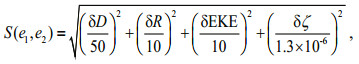
where δD, δR, δEKE, δζ are the distance and the differences in eddy radius, eddy kinetic energy, and vorticity between eddy e1 (in current time step t) and e2 (in next time step (t+δt), δt=1 day) of the same type (cyclonic or anticyclonic), respectively. The algorithm selects the eddy pair S(e1, e2) with minimal value and then considers this pair to be the same eddy that is tracked from t1 to t2 (Chaigneau et al., 2008).
The method of judging whether the two eddies refer to the same eddy is not based on the threshold value. It judges the same eddy as follows. When two similar eddies refer to the same eddy, the similar function will have a small value. For eddy e1 in time step t, the eddy e2 within searching radius L with the minimum similar function S(e1, e2) among eddies in time (t+δt) is regarded as the same eddy in consecutive time steps (Zhang et al., 2018; Dai et al., 2019). When no eddy is detected within searching radius in time t, the searching radius will extend to 1.5L in time (t+2δt) for extra searching as Nencioli et al. (2010) performed. If still no eddy detected, the detection of one eddy track is completed. The extra searching is conducted because eddies may vanish between successive SLA maps, particularly if they pass into the gaps between satellite ground tracks (Chaigneau et al., 2009). The searching radius L in this study is set as 50 km based on many factors, including eddy propagation speed (Chaigneau and Pizarro, 2005; Chelton et al., 2011), the accuracy error and spatial resolution of SLA data, and the risk of mismatching different eddies (Nencioli et al., 2010). We have selected 50 km as the searching radius, which indeed gives good eddy tracking results.
The eddy trajectories were obtained and numbered after tracking. After detecting and tracking, the eddy parameters were recorded or calculated, including the number, time, lifespan, type (cyclonic or anticyclonic), mean radius and amplitude, and the longitude and latitude of eddy centers and edges of eddies.
2.3 Methodology of colocalization and composite analysisMesoscale eddies possess the ability to carry a water mass in motion (Zhang et al., 2013). In order to characterize the drifter-carrying capability of mesoscale eddies, we implemented the algorithm of colocalization and composite analysis employed by de Marez et al. (2019). The algorithm of colocalization allows determining if a surface drifter lies inside or outside an eddy detected by the above algorithm. Every day, we seek all drifters collected. Then, for each eddy detected on this day, we check if a drifter is inside the eddy. If this condition is met, the drifter is flagged as "colocalized".
The dimensionless location related to the eddy center was computed for each colocalized drifter location. The dimensionless location comprises of the normalized radius λ and the azimuth θ. In Fig. 2, the normalized radius is defined as λ=d/a, where d is the distance between the eddy center and the drifter location, and a is the local radius of the eddy computed by finding the intersection between the eddy edge and a straight line that passes through the center of the eddy and the drifter position. If λ=0, the drifter is collected at the center of the eddy. If λ=1, the drifter is collected on the edge of the eddy. The azimuth θ increases counterclockwise from -180° (due west) to 180°.

|
| Fig.2 Normalized radius and azimuth a and b respectively show the calculation of the normalized radius of drifter D inside and outside the eddy, where E is the eddy center. As A is on the eddy edge, its normalized radius in the direction of ray ED is 1. The normalized radii of other points on the ray are calculated with reference to A. The drifter azimuth is positive in a but negative in b. |
The drifter-carrying processes of mesoscale eddies were named carrying processes that are defined in this paper as follows:
1) The drifter is under the influence of the eddy throughout the process (in this paper, we suppose that the influence range of the eddy is λ≤1.5).
2) At least one record of λ≤1 exists (i.e. the drifter has entered the eddy).
After colocalization, the normalized radius λ, and azimuth θ of each pair of eddies and drifters were calculated. Then, the carrying processes were extracted according to the above definition, and the following parameters were calculated: the carrying days (the number of days from the day when λ≤1 for the first time to the day when λ≤1 for the last time during the carrying process). The circles (the number of times the drifter completes moving around the eddy center during the carrying days) and the carrying distance (in this paper, it means the distance between the starting point and the end point of carrying days, e.g. the distance between A and B indicated by the black dashed line instead of the blue solid line in Fig. 3). It is noted that the large value of these three parameters reflect a strong drifter-carrying capability. The parameters along with λ and θ are known as carrying parameters. The circles are computed according to θ (which is of six-hourly temporal resolution) in the formula:


|
| Fig.3 Diagram of a carrying process The dots and irregular closed curves labeled with corresponding dates stand for the center and edge of a propagating eddy (No. 147333). The black dash-dotted line and the blue solid line indicate the trajectory of the eddy center and the drifter (No. 92981) during the carrying process respectively. The starting point A and the end point B indicate where the drifter starts to be carried and terminates being carried by the eddy. The black dashed line displays the distance between A and B. |
n stands for the carrying days,
in which the change of the azimuth per day is supposed no more than 180°. The circles mean the number of the circles that the drifter has completed moving around the eddy center during the carrying process.
Figure 3 demonstrates a carrying process of a cyclonic eddy occurred in the southwest of Honshu Island of eddy No. 147333 and drifter No. 92981, which last for 93 days. The distance between the starting point A and the end point B is 474 km (illustrated by the black dashed line) and the drifter made complete circles around the eddy center for about 7 times. It should be note that one eddy or one drifter may participate in more than one carrying process.
For a carrying process, when the drifter moves inside where λ≤1.5 (in this study) of the eddy, the normalized radius λ will change along with the time. When a drifter is closest to the eddy center, its normalized radius shall have the minimum value, the minimal λ is regarded as λ0, and the corresponding time (called relative time τ in this study) is set to be 0. Based on the relative time τ, the λ of carrying processes could be composited. In addition, λ0 reflects the degree that the drifter penetrates into the eddy during the carrying process.
Composite analysis is commonly utilized for the construction of eddy structures (Chaigneau et al., 2011; Ni, 2014; Dong et al., 2017; Zhang et al., 2018; Zhang and Qiu, 2018; Dai et al., 2019; de Marez et al., 2019; Yang et al., 2019). Assuming that all the eddies of the Peru-Chile Current System exhibit similar 3D structures, Chaigneau et al. (2011) employed composite analysis using a coordinate system (Δx, Δy) where each CTD profile is located respectively to the corresponding eddy center (Δx=Δy=0). Drifters in carrying processes localized relative to their corresponding eddy centers were investigated by a similar composite analysis using a coordinate system (λ, θ). Cyclonic eddies and anticyclonic eddies were studied respectively in composite analysis.
In order to examine the composite results in different locations, according to the previous study on the mesoscale eddies in the Pacific Ocean (Yang et al., 2013; Qiu et al., 2014; Zheng et al., 2014; Dong et al., 2017), the subregions were divided according to the latitude belongs to 0°–18°N, 18°N–25°N, 25°N–35°N, 35°N–42°N and 42°N–66°N, representing the tropical ocean (TO), the Subtropical Countercurrent (STCC), the Southern Kuroshio Extension (SKE), the Northern Kuroshio Extension (NKE), and the Subarctic Gyre (SAG) in the northwest Pacific, respectively. Figure 4 demonstrates the subregion division. We conducted the composite analysis for each subregion.

|
| Fig.4 The subregion division The study region is the northwest Pacific (99°E–180°E, 0°–66°N), which is divided into five subregions by the dashed red line, representing the tropical ocean (TO), the Subtropical Countercurrent (STCC), the Southern Kuroshio Extension (SKE), the Northern Kuroshio Extension (NKE), and the Subarctic Gyre (SAG) in the northwest Pacific, respectively |
The sea-surface velocity fields provided by the Copernicus Marine Environment Monitoring Service (CMEMS) for eddies were also composited for further study. A serial of preprocessing was done to realize this. Using the colocalization algorithm, the grid position (in longitude and latitude) of velocity field corresponding to an eddy is described with the coordinate system (λ, θ). Then we used the Data Interpolating Variational Analysis (DIVA) method (Troupin et al., 2012; see Section 2.6 in Dai et al., 2020; Song et al., 2019) to interpolate the velocity on an equal mesh-size grid. The velocity field for each eddy is thus convenient for composite.
3 STATISTICAL CHARACTERISTICS AND ANALYSIS OF CARRYING PROCESS 3.1 Basic statistical fact 3.1.1 Mesoscale eddyA total of 151 600 eddy trajectories were identified using the SLA of the northwest Pacific; of these 79 937 were cyclonic eddies and 71 663 were anticyclonic eddies (ratio of approximately 1.115:1). Figure 5 shows the sum of the numbers of eddy centers which passed through each 2°×2° square during the period 1993–2015. Both types of eddies are active in several areas, including the south and east of Taiwan, China, the south of Kyushu, the east of Honshu and Hokkaido, the vicinity of the Kuril Islands, the east of Kamchatka Peninsula, the southern Japan Sea, Attu Island (173°E, 53°N). The maximum values of both types were found to the east of the Korean Peninsula in the Japan Sea (130°E–132°E, 36°N–38°N): 6 954 cyclonic eddies and 7 495 anticyclonic eddies.

|
| Fig.5 The sum of the numbers of cyclonic eddy centers (a) and anticyclonic eddy centers (b) that passed through each 2°×2° square during 1993–2015 The squares in white stand for oceanic regions swallower than 200 m, where eddies are discarded due to significant aliases from tides and internal waves in SLA data there (Yuan et al., 2006). |
The frequency distribution of eddy lifespans is shown in Fig. 6. The numbers of both cyclonic and anticyclonic eddies decrease with an increase in eddy lifespan, but there are generally more cyclonic eddies than anticyclonic eddies. On average, the lifespan of cyclonic eddies is 16.67 days (maximum of 564 days) while that of anticyclonic eddies is 18.42 days (maximum of 1 306 days), which reveals that the lifespan of anticyclonic eddies is longer than that of cyclonic eddies (on average).

|
| Fig.6 Frequency distribution of eddy lifespans |
There were a total of 2036 drifters in the northwest Pacific between 1993 and 2015. Figure 7 demonstrates the sum of the number of drifters that passed through each 2°×2° square during 1993–2015. Drifter are active in the regions in the vicinity of the Kuroshio Current to the southeast of Taiwan, China, the southern Japan Sea (130°E–132°E, 36°N–38°N), which is also the region where eddies are most active) and south of the Kuroshio Extension. The statistics in these regions is more than 6 500 times. In the region south of the Kuroshio Extension (142°E–156°E, 26°N–34°N), almost all the 2°×2° squares have values of over 5 000. The statistics of drifters is related to the location of drifter deployment and distribution and the effect of the current.

|
| Fig.7 The sum of the numbers of drifters that passed through each 2°×2° square during 1993–2015 |
A total of 28 672 carrying processes were obtained by matching drifter data with eddy data, comprising 15 243 cyclonic processes and 13 429 anticyclonic processes (ratio of 1.135꞉1). It should be noted that the number of carrying process can be (in principle) larger than the number of drifters, because the same drifter would be carried by more than one eddy more than once. The sum of the numbers of the eddy centers of carrying processes that passed through each 2°×2° square is shown in Fig. 8.

|
| Fig.8 The sum of the numbers of the cyclonic eddy centers (a) and anticyclonic eddy centers (b) of carrying processes that passed through each 2°×2° square See Fig. 5 for the introduction of squares in white. |
As shown in Fig. 8, the statistics of cyclonic and anticyclonic eddies carrying processes is similar. The high-frequency carrying regions, such as the Kuroshio from the east of Luzon Island to the south of the Kuroshio Extension and the southern Japan Sea, are active regions of drifter and eddy. In addition, the carrying processes of cyclonic eddies are more frequent than anticyclonic processes in the region of the Subtropical Countercurrent (STCC), which is another region where carrying processes are active. For the extreme data, two squares of anticyclonic eddies have values over 90, but no squares of cyclonic eddy have such large number. The statistics of anticyclonic eddies carrying processes is denser than that of cyclonic eddies carrying processes, as all the local maxima of anticyclonic eddies carrying processes are larger than those of cyclonic eddies carrying processes. However, the total number of anticyclonic eddies carrying processes is lower than that of cyclonic eddies carrying processes.
The carrying days, circles, and carrying distances are the three significant indices representing the carrying capability of eddy. For cyclonic (anticyclonic) eddies, there are on average: 7.62 (7.61) carrying days, 0.31 (0.29) circles, and carrying distances of 101.9 (101.5) km. The maximum values for cyclonic (anticyclonic) eddies with respect to carrying days are 226 (182) days, circles of 22.39 (22.89), and carrying distance of 938.3 (906.8) km.
The frequency distributions of carrying days, circles, and carrying distances are shown in Fig. 9. The number of eddies decreases sharply with the increase of the number of carrying days and circles. The cyclonic (anticyclonic) carrying processes with less than 10 carrying days comprise 76.9% (76.5%) of the total cyclonic (anticyclonic) carrying processes. There are 95.5% cyclonic and anticyclonic eddies carrying processes with circles of less than one, and 95.5% and 95.9% of the cyclonic (anticyclonic) carrying processes have a carrying distance of less than 300 km.

|
| Fig.9 Frequency distribution of carrying days (a), circles (b), and carrying distances (c) |
Figure 10 illustrates the local maximum value of carrying days, circles, and carrying distances in each 2°×2° square. In detail, the value of one square is the maximum of one parameter of carrying processes originating in the square. Figure 10 concerns about the initial position of eddy center at the beginning of carrying processes with large value of carrying parameters, showing the differences in eddy carrying capability in different regions. For cyclonic eddies, the large values of circles are basically concentrated on the southern region of the Kuroshio Extension (140°E–160°E, 30°N–34°N), the eastern northwest Pacific (160°E–180°E, 18°N–36°N) and the Kuroshio region. It should be noted that some of the regions mentioned above are areas where eddies and drifters are active. For the anticyclonic eddies, large values of carrying days are scattered to the north of 20°N. In contrast to cyclonic eddies, there are fewer carrying days for anticyclonic eddies in the south of the Kuroshio Extension (140°E–160°E, 32°N–36°N). In addition, the maximum circles are distributed dispersedly. For the carrying distances, the region where the maxima of the anticyclonic eddies are mainly concentrated is located at around 23°N and 36°N, while that of the cyclonic eddies is located at around 18°N and 34°N.

|
| Fig.10 Local maximum values of carrying days (a and b), maximum circles (c and d), maximum carrying distances (e and f) of cyclonic eddies carrying processes (left panel) and anticyclonic eddies carrying processes (right panel) See Fig. 5 for the introduction of squares in white. |
The spatial distributions of carrying days, circles, and carrying distances are shown in Fig. 11. The trajectories of drifters carried are presented in different colors (which represent the values of carrying days, circles, and carrying distances of carrying processes). Figure 11 demonstrates the detailed trajectories of drifters during the carrying process with different carrying capability. The statistics comprehensively show the spatial diversity of the carrying capabilities. Most of the carrying processes have small values for these three parameters and they are widely distributed. Now we discuss the distributions of the three parameters respectively:

|
| Fig.11 Spatial distribution of carrying days (a and b), circles (c and d), and carrying distances (e and f) of cyclonic eddies carrying processes (left panel) and anticyclonic eddies carrying processes (right panel) See Fig. 4 for the meaning of the red dashed lines. |
(1) carrying days: the samples with the carrying days over 40 days are distributed densely in the SKE and the STCC (the NKE and the SAG) for cyclonic (anticyclonic) eddies. The carrying days of the major samples are less than 20 days in TO and mostly less than 10 days along the Kuroshio;
(2) circles: most of the cyclonic samples with number of circles more than 4 are densely located in the SKE, while the anticyclonic ones are scattered in the NKE and SAG. Most samples in the study region have circles less than 1;
(3) carrying distances: the cyclonic samples with the carrying distances over 400 km are distributed in the SKE and STCC, densely in the SKE in particular, and some are distributed in TO within 5°N–10°N, 125°E–150°E. The anticyclonic samples with the carrying days over 400 km are distributed in the NKE and STCC, not densely distributed as the cyclonic samples.
These results show that the carrying days, the circles, and the carrying distances represent different aspects of the carrying capability of eddies and they vary with the subregion and eddy type. 35°N seems to be a separatrix for the carrying capability of two types of eddies. It should be noted that the number of circles and the carrying distance do not always increase with an increase in the number of carrying days. If the eddy moves fast in one direction, the carrying process tends to have a small number of circles and a large carrying distance. In contrast, if the eddy moves slowly, the carrying distance tends to be small, and the number of circles depends on the rotational speed of the eddy.
The relationship between carrying days and circles of mesoscale eddies is shown in Fig. 12. Most of carrying days of the carrying processes are very short, as there are low numbers of both carrying days and circles. Overall, there is an increase in the number of circles with an increase in carrying days. Some carrying processes last for a long time; however, the number of circles does not increase accordingly, and this is explained in the discussion relating to Fig. 11. It is of note that for the same carrying days, there is an upper limit of the number of circles. At a preliminary estimate, circles ≤0.25×carrying days, which roughly reflects the upper limit of the rotational speed of the eddies. That is, in general, for particles rotating with the eddy for one day, the angle that they move around with respect to the eddy center does not exceed 90°.

|
| Fig.12 Scatter plot of relationship between circles and carrying days |
The 28 672 carrying processes were used as samples in a composite analysis of cyclonic eddies and anticyclonic eddies.
3.3.1 Relationship between minimum normalized radius and carrying processTo investigate the influence of the minimum normalized radius, λ0 on the carrying processes, the normalized eddy model is divided into four areas (area1, area2, area3, and area4), in accordance with λ belonging to (0, 0.25], (0.25, 0.5], (0.5, 0.75], and (0.75, 1], respectively. The area outside an eddy is area5. The carrying processes were grouped into 4 groups according to the smallest normalized radius λ0 belonging to (0, 0.25], (0.25, 0.5], (0.5, 0.75], and (0.75, 1], labeled g1, g2, g3, and g4, respectively. The statistical results here are in the whole region rather than in subregions.
Cyclonic eddies carrying processes are presented in Fig. 13, which shows the relative locations of drifters in all four groups and relative time τ from -40 to 40 (with an interval of 10). As shown in Fig. 13, with the smallest λ0 among the four groups (i.e. nearest to the eddy centers), λ0 of most drifters in g1 is within 0.75, when τ=-10 or τ=10. With an increase in absolute relative time, the drifters move outward; however, some are found to be within the eddies even at τ=-40 or τ=40. With respect to g4, the number inside eddies decreases sharply at τ=-20 or τ=20, and they are rare at τ=-30 or τ=30. Furthermore, the situation for g2 and g3 is found to be something between g1 and g4. Therefore, when the value of λ0 is smaller, the eddy has a stronger carrying effect on the drifter. A discussion about anticyclonic eddies is omitted because the results were similar to those of cyclonic eddies.

|
| Fig.13 Composite analysis of cyclonic eddies carrying processes The outer black circle represents λ=1.5, and the inner black circle represents λ=1.0. The drifters are grouped into 4 groups named g1–g4 according to λ0 when τ=0. As τ=0 is the origin of time, the drifters are rigidly distributed in the best order within their areas of origin. With an increase in absolute relative time, the number of drifters inside eddies tends to decrease, and the distribution of drifters lacks order. |
Figure 14 shows the number of g1 (cyclonic eddies marked in black in Fig. 13) in area1–area5 varying with relative time. Away from τ=0, the summits of the number of drifters appear in turn from area1–area4 in the adjacent relative time, which indicates that the majority of drifters approach and leave the eddy center rapidly (and the situation for g2–g4 is similar). The numbers of the entire cyclonic eddies carrying processes in area1–area5 varying with relative time are counted in Fig. 15, and again shows that the drifters approach and leave eddies rapidly. Reporting details of the anticyclonic situation is unnecessary here, as it is similar to that of the cyclonic situation.

|
| Fig.14 Numbers of g1 of cyclonic eddies carrying processes in area1–area5 varying with relative time τ Circles and numbers in figure indicate relative time and number of drifters in each area at summits. |

|
| Fig.15 Numbers of entire cyclonic eddies carrying processes in area1–area5 varying with relative time τ |
The average carrying days were investigated for different regions, eddy types, and groups. Table 1 is sample numbers and corresponding averaged carrying days in detail.
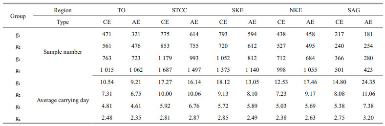
The average carrying days of both cyclonic and anticyclonic eddies in TO and the STCC are similar, while in the SKE, the average carrying days of cyclonic eddies are larger than that of anticyclonic eddies, and it is on the contrary for the NKE and the SAG (Table 1). It shows that, on average, in TO and the STCC, opposite types of eddies have similar carrying capability, while in the SKE the cyclonic eddies have stronger carrying capability and in the NKE and the SAG the anticyclonic eddies have stronger carrying capability. It reveals the fact that the carrying capability may be different for different regions and different types of eddies.
3.3.2 Relationship between average normalized radius and carrying daysIn order to find the similarity and difference of the variation in different regions and of different carrying days, we grouped the samples by relative time τ. The carrying processes with min (max (τ), |min (τ)|)≥15 are grouped into d5. In the rest samples, the one whose min (max (τ), |min (τ)|)≥12 are grouped into d4. In the same way, min (max (τ), |min (τ)|)≥9, min (max (τ), |min (τ)|)≥6 and min (max (τ), |min (τ)|)≥3 are grouped into d3, d2, and d1, respectively. The carrying days of the samples are increasing from d1 to d5, reflecting that the carrying capability of the eddies are strengthening. The normalized radii in each subregion and each group were averaged by the sample number with the same relative time τ.
Figure 16 displays the average normalized radius λ varying with the relative time τ. In each group, the variation of normalized radius λ shares the common trends, i.e. with the increase of relative time τ, the average normalized radii mostly decrease to the minimum when τ=0, and then increase, meaning that the drifter would approach the eddy center and then leave away from it. However, it should be noted that mostly when the carrying days are large (≥9 days, i.e. d3 to d5 in the paper), there is a relatively slow variation of λ with the increase or decrease of the relative time from τ=0. When the average normalized radius varies slowly, the relative time interval is called a slowly-varying interval. Averaging the average normalized radius during the slowly-varying interval thus provides a value referred to as the slowly-varying radius. Of course, the slowly-varying radius in some parts of the Fig. 16 is not so obvious. This shows that, on average, when the carrying days are large, drifters tend to travel for longer time on around certain normalized eddy radii during a carrying process. In statistics, the normalized eddy radii range from 0.41– 0.76. However, it is acknowledged that this conclusion may be influenced by the limited sample size employed. The results also show that when λ0 is smaller, the drifters move deeper into eddies, and the number of carrying days is therefore longer.

|
| Fig.16 Relationship between average normalized radius λ and relative time τ of cyclonic eddies (left panel) and anticyclonic eddies (right panel) The red line represents the averaged normalized radius and the blue dashed line displays the slowly-varying radius. The sample number for each subfigure lies on the top right corner. Some subfigures do not contain the blue dashed line because the slowly-varying radius is not obvious of corresponding groups. Only d3–d5 are displayed for the same reason. d5 of cyclonic eddies carrying processes in SAG is absent for no sample. |
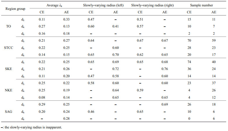
Table 2 lists the λ0 and the slowly-varying radius. On sample number, with the exception of NKE, the sample number of cyclonic eddy is larger than that of anticyclonic eddy. The average λ0 of two types of eddies are similar in general for each region and each group and the corresponding slow-varying radius of anticyclonic eddy is larger than cyclonic eddy in general.
The carrying capability of eddies in different regions is different and the mechanism is somewhat complicated. Mesoscale eddies are in geostrophic balance due to the Earth rotation to a lowest order, but the ageostrophic motion is significant to the dissipation of the eddies (Zhang and Qiu, 2018). The pure geostrophic current, which flows along the contour line of SLA, will drive particles to travel along the SLA contours. Thus, the entrance and exit of the drifters result from the ageostrophic velocity. In order to describe the ageostrophic effect, we have introduced the Rossby number (Zhang et al., 2015) to investigate its relation with the carrying capability. The larger is the Rossby number, the weaker the geostrophic effect, and the smaller the Coriolis force compared with the inertial force (Cushman-Roisin and Beckers, 2011), in which the geostrophic balance can no longer be held (Zhang and Qiu, 2018).
In this study, the Rossby number is defined as
Ro=U/fr,
where U is the maximum velocity among the composited eddy velocity field, r the radius and f the Coriolis parameter related to latitude, reflecting the combined influence of the velocity field, radius and latitude of an eddy. It is noted that U, f, and r are averaged by relative time τ range from -3‒3, -6‒6, -9‒9, -12‒12 and -15‒15 of d1‒d5, respectively.
The carrying days of the samples are increasing from group d1 to d5, which means that the carrying capability is strengthening correspondingly. Figure 17 displays the Rossby number of each region and eddy type, from which the Rossby number decrease in general with the increase of the carrying days. The conclusion was drawn that eddies with smaller Rossby number tend to have stronger drifter-carrying capability on average. In detail for example, for cyclonic eddies in the STCC, when the Ro≤0.016, the carrying days are more than 9 days. The fact is acceptable considering the meaning of Rossby number, which reflects the ratio of the ageostrophic motion to the geostrophic motion. When the Rossby number is small, the motion is nearly geostrophic. The drifter would travel along the contour of SLA, carried by the eddy for longer time. Small maximum velocity, large Coriolis parameter, and large radius contribute to the carrying capability. On the contrary, when the Rossby number is large, ageostrophic component increases. The drifter would travel through the SLA contour. The motion is instable leading to small carrying days. In addition, comparing the Rossby number of eddies in two types, the value of cyclone is larger (slightly smaller) than the value of anticyclone in the south (north) of 35°N in each group, respectively.

|
| Fig.17 Rossby number of each group in each region of cyclonic eddies (a) and anticyclonic eddies (b) |
In this paper, we considered the drifters as real particles to characterize the carrying capability of mesoscale eddy. By combining the SLA data and the drifter data in the northwest Pacific (99°E–180°E, 0°–66°N) from 1993 to 2015, the statistical characteristics of carrying particles for mesoscale eddies were revealed by the method of colocalization and composite analysis. Rossby number is introduced to interpret the eddy's carrying capability variation. The conclusions made are as follows:
(1) The motion of carried drifters reflects the upper limit of rotational speed of eddies. According to the relationship between carrying days and number of circles (the number of circles the drifter revolving around the eddy center), a preliminary estimation is that the number of circles are ≤0.25 × carrying days (i.e. in most cases, the particles move no more than 90° around the eddy center when carried by an eddy for one day).
(2) The number of carrying days is related to the smallest normalized radius between the drifter and eddy center. According to the composite analysis, during the carrying process, when the normalized radius is smaller, the carrying days tend to be longer and the eddies tend to have a stronger carrying effect on drifters.
(3) In different subregions, the carrying capability of cyclonic and anticyclonic eddies is different. The composite analysis was conducted in subregions. On average, in TO and the STCC, opposite types of eddies have similar carrying capability, while in the SKE the cyclonic eddies tend to have stronger carrying capability and in the NKE and SAG the anticyclonic eddies tend to have stronger carrying capability.
(4) On average, when the carrying days are large (≥9 days in the paper), drifters tend to travel for longer time in around certain normalized eddy radii during a carrying process. In statistics, the normalized eddy radii range from 0.41–0.76.
(5) The carrying capability has a close relation with the Rossby number of the eddy that small Rossby number corresponds to large carrying days in general, and the carrying days reflect the carrying capability of eddies. The current is closer to geostrophic flow in large Rossby numbers and the drifter would travel nearly along the contour of SLA, carried by the eddy for longer time.
5 DATA AVAILABILITY STATEMENTThe datasets generated and analyzed during the current study are available from the corresponding author on reasonable request.
6 ACKNOWLEDGMENTWe sincerely appreciate two reviewers and Dr. ZHANG Zhengguang for detailed and valuable suggestions. The eddy identification and tracking program is from Dr. NI Qinbiao. The altimeter products used in this study are distributed by Archiving Validation and Interpretation of Satellite Data in Oceanography (AVISO), the Centre National d'Études Spatiales (CNES) of France (http://www.aviso.altimetry.fr/en/data/products/sea-surface-heightproducts/global.html), the drifter data are provide from National Oceanic and Atmospheric Administration (NOAA) (https://www.aoml.noaa.gov/phod/gdp/hourly_data.php) and the geostrophic velocity anomaly data were provided by the Copernicus Marine Environment Monitoring Service (CMEMS) (http://marine.copernicus.eu/).
Chaigneau A, Eldin G, Dewitte B. 2009. Eddy activity in the four major upwelling systems from satellite altimetry (1992-2007). Progress in Oceanography, 83(1-4): 117-123.
DOI:10.1016/j.pocean.2009.07.012 |
Chaigneau A, Gizolme A, Grados C. 2008. Mesoscale eddies off Peru in altimeter records: identification algorithms and eddy spatio-temporal patterns. Progress in Oceanography, 79(2-4): 106-119.
DOI:10.1016/j.pocean.2008.10.013 |
Chaigneau A, Le Texier M, Eldin G, Grados C, Pizarro O. 2011. Vertical structure of mesoscale eddies in the eastern South Pacific Ocean: a composite analysis from altimetry and Argo profiling floats. Journal of Geophysical Research: Oceans, 116(C11): C11025.
DOI:10.1029/2011JC007134 |
Chaigneau A, Pizarro O. 2005. Eddy characteristics in the eastern South Pacific. Journal of Geophysical Research: Oceans, 110(C6): C06005.
|
Chelton D B, Schlax M G, Samelson R M. 2011. Global observations of nonlinear mesoscale eddies. Progress in Oceanography, 91(2): 167-216.
DOI:10.1016/j.pocean.2011.01.002 |
Cushman-Roisin B, Beckers J M. 2011. Quasi-geostrophic dynamics. International Geophysics, 101: 521-551.
DOI:10.1016/B978-0-12-088759-0.00016-X |
Dai J, Wang H Z, Zhang W M, An Y Z, Zhang R. 2020. Observed spatiotemporal variation of three-dimensional structure and heat/salt transport of anticyclonic mesoscale eddy in Northwest Pacific. Journal of Oceanology and Limnology.
DOI:10.1007/s00343-019-9148-z |
de Marez C, L'Hégaret P, Morvan M, Carton X. 2019. On the 3D structure of eddies in the Arabian Sea. Deep Sea Research Part I: Oceanographic Research Papers, 150: 103057.
DOI:10.1016/j.dsr.2019.06.003 |
Dong C M, Liu Y, Lumpkin R, Lankhorst M, Chen D K, McWilliams J C, Guan Y P. 2011. A Scheme to Identify Loops from Trajectories of Oceanic Surface Drifters: An Application in the Kuroshio Extension Region. Journal of Atmospheric and Oceanic Technology, 28(9): 1167-1176.
DOI:10.1175/JTECH-D-10-05028.1 |
Dong D, Brandt P, Chang P, Schütte F, Yang X F, Yan J H, Zeng J S. 2017. Mesoscale eddies in the Northwestern Pacific Ocean: three-dimensional eddy structures and heat/salt transports. Journal of Geophysical Research: Oceans, 122(12): 9795-9813.
DOI:10.1002/2017JC013303 |
Duo Z J, Wang W K, Wang H Z. 2019. Oceanic mesoscale eddy detection method based on deep learning. Remote Sensing, 11(16): 1921.
DOI:10.3390/rs11161921 |
Jia Y L, Liu Q Y. 2004. Eddy shedding from the Kuroshio Bend at Luzon strait. Journal of Oceanography, 60(6): 1063-1069.
DOI:10.1007/s10872-005-0014-6 |
Li J X, Wang G H, Xue H J, Wang H Z. 2019. A simple predictive model for the eddy propagation trajectory in the northern South China Sea. Ocean Science, 15(2): 401-412.
DOI:10.5194/os-15-401-2019 |
Li J X, Zhang R, Jin B G. 2011. Eddy characteristics in the Northern South China Sea as inferred from Lagrangian drifter data. Ocean Science, 7(5): 661-669.
DOI:10.5194/os-7-661-2011 |
Lumpkin R, Grodsky S A, Centurioni L, Rio M H, Carton J A, Lee D. 2013. Removing Spurious Low-Frequency Variability in Drifter Velocities. Journal of Atmospheric and Oceanic Technology, 30(2): 353-360.
DOI:10.1175/JTECH-D-12-00139.1 |
Lumpkin R, Pazos M. 2007. Measuring surface currents with Surface Velocity Program drifters: the instrument, its data, and some recent results. In: Griffa A, Kirwan Jr A D, Mariano A J, Özgökmen T, Rossby H T eds. Lagrangian Analysis and Prediction of Coastal and Ocean Dynamics. Cambridge University Press, Cambridge. p.39–67.
|
Nencioli F, Dong C M, Dickey T, Washburn L, McWilliams J C. 2010. A vector geometry-based eddy detection algorithm and its application to a high-resolution numerical model product and high-frequency radar surface velocities in the southern California Bight. Journal of Atmospheric and Oceanic Technology, 27(3): 564-579.
DOI:10.1175/2009JTECHO725.1 |
Ni Q B. 2014. Statistical Characteristics and Composite Three-dimensional Structures of Mesoscale Eddies near the Luzon Strait. Xiamen University, Xiamen.
(in Chinese with English abstract) |
Niiler P P, Sybrandy A S, Bi K, Poulain P M, Bitterman D. 1995. Measurements of the water-following capability of holey-sock and tristar drifters. Deep Sea Research. Part I: Oceanographic Research Papers, 42(11-12): 1951-1964.
DOI:10.1016/0967-0637(95)00076-3 |
Niiler P. 2001. The world ocean surface circulation. International Geophysics, 77: 193-204.
DOI:10.1016/S0074-6142(01)80119-4 |
Qiu B, Chen S M, Klein P, Sasaki H, Sasai Y. 2014. Seasonal Mesoscale and Submesoscale eddy variability along the North Pacific subtropical countercurrent. Journal of Physical Oceanography, 44(12): 3079-3098.
DOI:10.1175/JPO-D-14-0071.1 |
Rio M H. 2012. Use of altimeter and wind data to detect the anomalous loss of SVP-type drifter's drogue. Journal of Atmospheric and Oceanic Technology, 29(11): 1663-1674.
DOI:10.1175/JTECH-D-12-00008.1 |
Song B, Wang H Z, Chen C L, Zhang R, Bao S L. 2019. Observed subsurface eddies near the Vietnam coast of the South China Sea. Acta Oceanologica Sinica, 38(4): 39-46.
DOI:10.1007/s13131-019-1412-8 |
Souza J M A C, de Boyer Montégut C, Le Traon P Y. 2011. Comparison between three implementations of automatic identification algorithms for the quantification and characterization of mesoscale eddies in the South Atlantic Ocean. Ocean Science, 7(3): 317-334.
DOI:10.5194/os-7-317-2011 |
Troupin C, Barth A, Sirjacobs D, Ouberdous M, Brankart J M, Brasseur P, Rixen M, Alvera-Azcárate A, Belounis M, Capet A, Lenartz F, Toussaint M E, Beckers J M. 2012. Generation of analysis and consistent error fields using the data interpolating variational analysis (DIVA). Ocean Modelling, 52-53: 90-101.
DOI:10.1016/j.ocemod.2012.05.002 |
Wang G H, Su J L, Chu P C. 2003. Mesoscale eddies in the South China Sea observed with altimeter data. Geophysical Research Letters, 30(21): 2121.
DOI:10.1029/2003GL018532 |
Wang H Z, Guo P, Ni Q B, Li J X. 2018. A CFSFDP clustering-based eddy trajectory tracking method. Acta Oceanologica Sinica, 40(8): 1-9.
(in Chinese with English abstract) |
Wang H Z, Liu Q H, Yan H Q, Song B, Zhang W M. 2019a. The interactions between surface Kuroshio transport and the eddy field east of Taiwan using satellite altimeter data. Acta Oceanologica Sinica, 38(4): 116-125.
DOI:10.1007/s13131-019-1417-3 |
Wang Z F, Sun L, Li Q Y, Cheng H. 2019b. Two typical merging events of oceanic mesoscale anticyclonic eddies. Ocean Science, 15(6): 1545-1559.
DOI:10.5194/os-15-1545-2019 |
Yang G, Wang F, Li Y L, Lin P F. 2013. Mesoscale eddies in the northwestern subtropical Pacific Ocean: statistical characteristics and three-dimensional structures. Journal of Geophysical Research: Oceans, 118(4): 1906-1925.
DOI:10.1002/jgrc.20164 |
Yang Z B, Wang G H, Chen C L. 2019. Horizontal velocity structure of mesoscale eddies in the South China Sea. Deep Sea Research Part I: Oceanographic Research Papers, 149: 103055.
DOI:10.1016/j.dsr.2019.06.001 |
Yuan D L, Han W Q, Hu D X. 2006. Surface Kuroshio path in the Luzon Strait area derived from satellite remote sensing data. Journal of Geophysical Research: Oceans, 111(C11): C11007.
DOI:10.1029/2005JC003412 |
Zhang W Z, Ni Q B, Xue H J. 2018. Composite eddy structures on both sides of the Luzon Strait and influence factors. Ocean Dynamics, 68(11): 1527-1541.
DOI:10.1007/s10236-018-1207-z |
Zhang W Z, Xue H J, Chai F, Ni Q B. 2015. Dynamical processes within an anticyclonic eddy revealed from Argo floats. Geophysical Research Letters, 42(7): 2342-2350.
DOI:10.1002/2015GL063120 |
Zhang Z G, Qiu B. 2018. Evolution of submesoscale ageostrophic motions through the life cycle of oceanic mesoscale eddies. Geophysical Research Letters, 45(21): 11847-11855.
DOI:10.1029/2018GL080399 |
Zhang Z G, Wei W, Bo Q. 2014. Oceanic mass transport by mesoscale eddies. Science, 345(6194): 322-324.
DOI:10.1126/science.1252418 |
Zhang Z G, Zhang Y, Wang W, Huang R X. 2013. Universal structure of mesoscale eddies in the ocean. Geophysical Research Letters, 40(14): 3677-3681.
DOI:10.1002/grl.50736 |
Zheng C C, Yang Y X, Wang F M. 2014. Spatial-temporal features of eddies in the North Pacific. Marine Sciences, 38(10): 105-112.
(in Chinese with English abstract) |